In each training step, one sample vector ![]() from the input data
set is chosen randomly and a similarity measure is calculated between
it and all the weight vectors of the map. The Best-Matching Unit
(BMU), denoted as c, is the unit whose weight vector has the
greatest similarity with the input sample
from the input data
set is chosen randomly and a similarity measure is calculated between
it and all the weight vectors of the map. The Best-Matching Unit
(BMU), denoted as c, is the unit whose weight vector has the
greatest similarity with the input sample ![]() . The similarity is
usually defined by means of a distance measure, typically Euclidian distance.
Formally the BMU is defined as the neuron for which
. The similarity is
usually defined by means of a distance measure, typically Euclidian distance.
Formally the BMU is defined as the neuron for which
![]()
where ![]() is the distance measure.
is the distance measure.
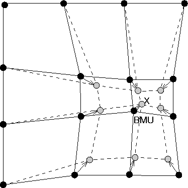
After finding the BMU, the weight vectors of the SOM are updated. The weight vectors of the BMU and its topological neighbors are moved closer to the input vector in the input space. This adaptation procedure stretches the BMU and its topological neighbors towards the sample vector. This is illustrated in figure 2.2, where the input vector given to the network is marked by an x.

Figure 2.2: Updating the best matching unit (BMU) and its
neighbors towards the input sample marked with x.
The solid and dashed lines correspond to situation before and after
updating, respectively.
The SOM update rule for the weight vector of the unit i is:
![]()
where t denotes time. The ![]() is the input
vector randomly drawn from the input data set at time t and
is the input
vector randomly drawn from the input data set at time t and
![]() the neighborhood kernel around the winner unit c at time
t. The neighborhood kernel is a non-increasing function of time and of
the distance of unit i from the winner unit c. It defines the
region of influence that the input sample has on the SOM. The kernel
is formed of two parts: the neighborhood function h(d,t) and the learning
rate function
the neighborhood kernel around the winner unit c at time
t. The neighborhood kernel is a non-increasing function of time and of
the distance of unit i from the winner unit c. It defines the
region of influence that the input sample has on the SOM. The kernel
is formed of two parts: the neighborhood function h(d,t) and the learning
rate function ![]() :
:
![]()
where ![]() is the location of unit i on the map grid.
is the location of unit i on the map grid.
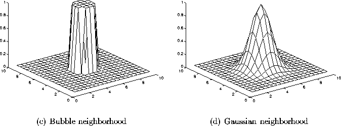
The simplest neighborhood function is the bubble: it is constant over
the whole neighborhood of the winner unit and zero elsewhere (see
figure 2.3a). Another is the Gaussian neighborhood
function ![]() (see figure 2.3b). It gives slightly better results but is
computationally somewhat heavier. Usually the neighborhood radius is
bigger at first and is decreased linearly to one during the training.
(see figure 2.3b). It gives slightly better results but is
computationally somewhat heavier. Usually the neighborhood radius is
bigger at first and is decreased linearly to one during the training.

Figure 2.3: The two basic neighborhood functions.
The learning rate ![]() is a decreasing function of time. Two
commonly used forms are a linear function and a function
inversely proportional to time:
is a decreasing function of time. Two
commonly used forms are a linear function and a function
inversely proportional to time: ![]() ,
where A and B are some suitably selected constants. Use
of the latter function type ensures that all input samples
have approximately equal influence on the training
result [31].
,
where A and B are some suitably selected constants. Use
of the latter function type ensures that all input samples
have approximately equal influence on the training
result [31].
The training is usually performed in two phases. In the first phase, relatively large initial alpha value and neighborhood radius are used. In the second phase both alpha value and neighborhood radius are small right from the beginning. This procedure corresponds to first tuning the SOM approximately to the same space as the input data and then fine-tuning the map. If the linear initialization procedure is used the first training phase can be skipped. There are several rules-of-thumb, found through experiments, for choosing suitable values [21].
There are many variants to the basic SOM. One variantion theme is to use neuron-specific learning rates and neighborhood sizes. Another is to use adaptive or even growing map structures. The goal of these variations is to enable the SOM to follow better the topology of the underlying data set or to achieve better quantization results. An usual defect of these methods is that the visualization properties suffer or that the algorithm becomes computationally heavier.