Exercises

Back to course page.

The exercise problems will be added here after each session. You should return your solution to the assistant within two weeks from the time the exercise was given. You can (and are encouraged to) use suitable tools for solving the exercises, so please use Matlab or something like that instead of inverting 6x6 matrices by hand. If solving the problem using computer then return the code and the key results. Otherwise it is completely okay to return also hand-written solutions.

9.3.

This exercise concerns the latter paper I presented. You will need information in Sections 2 and 3 to solve the exercise.

You have 6 proteins, named A,B,C,D,E and F. You already know the interactions between A,B and C (group 1) and wish to know interactions between group 1 and proteins D,E,F (group 2), as well as interactions within group 2.

Adjacency list of group 1 (known):
A: C
B: C
C: A,B

Part 1.

Compute protein interaction network kernel estimate Q based on the noisy interaction data given below. For this you will need to create diffusion kernels for both the known network and the data, and then compute Q using those. What do the different parts of matrix Q tell? How would you obtain a list of links between the proteins from this?

Adjacency list for noisy data:
A: B,C,D
B: A,C,F
C: A,B,C,D,E,F
D: A,C,E
E: C,D,F
F: B,C,E

Edit (19.3.2007): Added F to the adjacency list of C to make the graph undirected. If you already did the exercise with the old version it is naturally perfectly okay.

Hint: In Matlab exp() is elementwise exponentiation. To exponentiate a matrix use expm().

Part 2.

You're additionally given an expression level data with six experiments for each of the proteins. Generate kernel matrix from the data given below, using a kernel of your choice, and combine it with the noisy data from part 1. Again estimate Q, but instead of using the EM-algorithm described in the paper use weight 0.3 for the first data and 0.7 for this one. Does the result differ much from the first part?

Expression levels:
A: -0.1511    1.4386   -0.1026    0.2815   -0.0529    1.0592
B:  0.0928   -1.1930   -0.1320   -0.4606   -0.1442   -0.3411
C:  0.3785    1.5472   -0.1913    0.7036   -0.1101    1.0223
D: -0.3901    1.2165   -0.0401    0.1166    0.0012    0.9270
E: -0.5895    0.8906    0.4040    0.1305    0.1900    0.7915
F:  0.1024    0.6988    0.0078    0.3268    0.1278    0.6700

You can assume that all expression measurements are from very similar probes so you can assume they all have the same variance.

If you want to know more about the kernels you can check this paper and the video-lecture. These are not needed for the exercise as such.

16.3.

Part 1. Simulate (in Matlab or whatever) one realization of Erdos-Renyi -network with 1000 nodes and p=0.1. Calculate degree distribution p(k) for that network and plot it.

Part 2. Simulate one realization of Barabasi-Albert -network model with 10000 nodes and m=1 (that is, add one link when adding each node). Use network with two connected nodes as a seed network. Calculate degree distribution p(k) for that network and plot it using log-log scale.

Hint: It is probably good idea to store the links in a sparse matrix. If you cannot create a network with 10000 nodes (because of memory constraints) then create a smaller one.

Part 3. What distributions do these degree distributions resemble?

23.3.

See this file for the exercise problem.

30.3. (added at 13.4.)

What are the main assumptions made for module networks to alleviate the modeling problem? How about the MinReg model? For module networks you may need to look Sections 2 and 3, and for MinReg Section 2.

Compare the assumptions. Does either one make more sense to you, or do they fit to different kind of situations? The MinReg paper has some arguments in favor of their model in comparison to the module networks (Section 4.3.1 and the last paragraph of Section 5). Do you agree with them? Do module networks have some advantages over MinReg (a MinReg-paper might not list such points)?

13.4. (added 16.4.)

Note: the exercise may look like a long one, but it should not be that complicated. If it still seems to take too long, just stop at some point and explain how you would have done the rest.

You have a fully observed time series about three variables: A, B, and C. The data is in abc.dat where each row represents a time step and there's a column for each variable (A,B,C respectively). Each variable has 3 values. For your convenience, the values are labeled "1", "2" and "3", so that indexing tables will be easy (at least in Matlab). Hint: in Matlab "D = load('abc.dat')" reads the data in.

We can assume each variable depends on it's own previous value, so that the A(t-1) is a parent of A(t) etc. Your ultimate task is to find more parents for the variable A: as if A was the target gene and B and C were the potential regulators.

Part 1: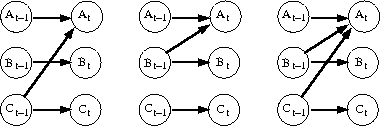

Find the maximum likelihood estimate for the parameters of the three DBN models in the above figure. This can be done simply by counting (into 2-, 3-, or 4-dimensional tables) how many times the variables have each of their combinations and finally normalising the counts so that they obey the properties of conditional probability distributions. E.g. P(A(t) | A(t-1), B(t-1)) sums up to one for each combination of the parent variables: in Matlab "sum(P_AAB(:,a,b)) == 1" for each (a,b) in A(t-1) x B(t-1.)

Note that the estimate of prior probabilities is based only on the first time step and conditional probabilities are based on time steps 2 through T.

Part 2:

Compute the logarithmic likelihood of the data for each model using the estimated probabilities. Hint: ln(P(A(1:T), B(1:T), C(1:T)) decomposes nicely because of the product rule of the given Bayes net, and you can leave out terms that are identical for all three models if you want to (no need to estimate them in the first part either).

Part 3:

Compute the BIC score for each of the three models: BIC = ln(P(A(1:T), B(1:T), C(1:T)) - 0.5 * #G * ln T, where T is the number of time steps and #G is the number of parameters in each of the models (don't forget the priors). For example P(C(t) | C(t-1)) has 3*3 = 9 parameters.

Which of the models has the highest score? What if we ranked them using the log. likelihood only? Finally, which of the potential regulators (B and C) affect the activity of the gene A?

20.4.

See this file for the exercise problem.

27.4.

Answer briefly to the following questions based on the first presentation of the day:

1. What are the main steps in construction models of metabolic networks?

2. Why models estimated as described in this paper are usually inconsistent with experimental data, and how this can be corrected?