
Laboratory of Computer and Information Science > Teaching > T-61.5060 > Exercises 2007 > Solutions 2
% getSpBinData is not a public Matlab function
A = getSpBinData('abstracts10000.txt');
% Now matrix A is a binary matrix with documents as rows
% and words as columns. A matrix element (i,j) is 1 iff
% document i contains the word j.
wordOcc = full(sum(A));
wordOcc = nonzeros(wordOcc);
words = length(wordOcc);
wordOcc = sort(wordOcc, 'descend');
ly = log(wordOcc);
lx = [ ones(words,1), log(1:words)' ];
% The backslash command solves a general linear equation.
% In cases like this one, it gives out the least squre error
% solution.
coeffs = lx \ ly;
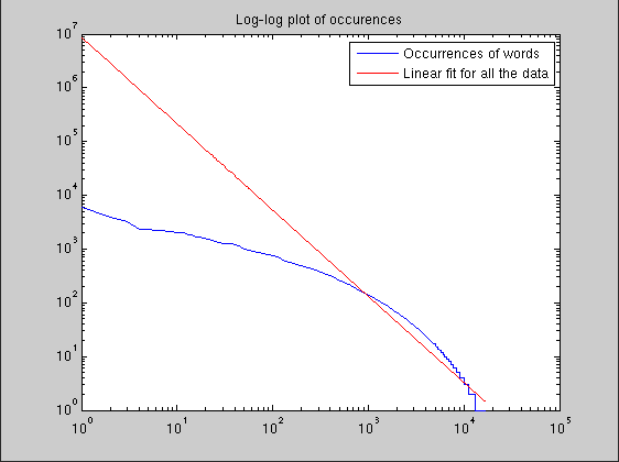
loglog(1:words, wordOcc);
hold on;
plot(exp(lx(:,2)), exp(lx*coeffs), 'r');
title('Log-log plot of occurences');
legend('Occurrences of words', 'Linear fit for all the data');
This gives f(k) approx exp(16)*k^(-1.6). (coeffs = [ 15.96, -1.601 ])
close all;
rows = randint(1000,1, [1, 10000]);
sampleOcc = nonzeros(full(sum(A(rows,:))));
sampleOcc = sort(sampleOcc, 'descend');
thOcc = exp(16)*(1:length(sampleOcc)).^(-1.6)/10; % 10 = 10000/1000
% Pretty uninteresting plots.
loglog(sampleOcc);
hold on;
plot(thOcc);


% Just run this function. Every time it gives a comparison between
% random real data occurrence and fitted occurrence values.
function test(sampleOcc, thOcc)
	ind = randint(1,1,[1, length(sampleOcc)]);
	disp(sprintf('Sample has: %dth count is %d', ind, sampleOcc(ind)));
	disp(sprintf('Approximation gives: %dth count is %.2f', ind, thOcc(ind)));
	disp(' ');
end
The leftmost approximations are very poor, but as the lower tail counts are much more common, the fitting also prefers that area.
SHELL > ./apriori abstract10000.txt 3 2000 out.txt
...
1 16644 10000 [0.27s] 11 [0s]
2 8212 [0.16s] 1 [0s]
...
Now we just type
SHELL > tail -1 out.txt
21614 23313 (2213)
SHELL > grep -P "21614|23313" words.txt
21614 project
23313 research
And that's it.
Binomial distribution is nothing but a sum of samples from the one and the same Bernoulli distribution. That means that it will surely converge to a normal distribution, when n is sufficiently large.
The mean and variance of the binomial distribution are np and np(1-p).
Thus N(np, np(1-p)), is a good approximation for it and used usually
when np, np(1-p) > 5 or 10. Note that
P(Bin(n,p) <= X) approx P(N(np, np(1-p)) <= X + 0.5)
Poisson distribution is used to model a Poisson process, a process where events happen in approximately constant intervals lambda. It is pretty obvious that this description fits also the binomial distribution, at least when p is small enough so that the discreteness doesn't blow up things. Poisson(np) has mean np and variance np, and it is very close to Bin(n,p) when n is large, p is small and hopefully np remains pretty much a constant.
Second to last row: Even though the hash functions are not probably independent of each other, we here assume that these inequalities are! What's going on? The point is that the hash functions may be dependent conditional on some certain data, but on general situation as this one here, they all are bound with the same requirement of 2-universal hash function family: smooth dispersion. Thus the general data-independent probabilities for the cell sizes are actually still independent of each other and thus we can break this probability into a intersection (or a product).
Take epsilon = 10^(-5), delta = 10^(-2). This implies w = 271829 and d = 5, so we need a table of 1,4 million cells, that is something like 6 megabytes. If we receive S = 10 million packets during the day then only 1 percent of the packet amount approximations will have an error larger than epsilon*S = 100.
<Set size> <Random obfuscated, non-documented foo> <Number of found sets>Output text file has form
<Elements of the set> (<Support of the set>)
SHELL > ./apriori abstracts10000.txt 3 300 out.txt
Apriori frequent itemset mining implementation
by Bart Goethals, 2000-2003
http://www.cs.helsinki.fi/u/goethals/

1 16644 10000 [0.27s] 434 [0s]
2 9996 [1.67s] 734 [0.02s]
3 2164 [0s] 8957 [0.35s] 172 [0.01s]
4 35 [0s] 2238 [0.21s] 7 [0s]
5 0 [0s] 0 [0.21s] 0 [0s]

1347    [2.74s]
Frequent sets written to out.txt

SHELL > tail -7 out.txt
21614 23313 24416 29137 (312)
21582 21614 23313 24416 (326)
1967 23313 26977 29137 (381)
21614 23313 26977 29137 (301)
1967 21582 23313 29137 (322)
1967 21614 23313 29137 (327)
21582 21614 23313 29137 (371)
You are at: CIS → T-61.5060 Exercises 2007, Solutions 2
Page maintained by t615060@james.hut.fi, last updated Monday, 15-Oct-2007 18:23:35 EEST