Tik-61.261 Principles of Neural Computing
Raivio, Venna

Exercise 5,

1. The McCulloch-Pitts perceptrons can be used to perform numerous logical tasks. Neurons are assumed to have two binary input signals, $x_1$ and $x_2$, and a constant bias signal which are combined into an input vector as follows: $\mathbf{x}=[x_1,x_2,-1]^T$, $x_1,x_2\in \{0,1\}$. The output of the neuron is given by

   $$y=\begin{cases}1 \text{, \, if } \mathbf{w}^T\mathbf{x}>0 \\ 0 \text{, \, if } \mathbf{w}^T\mathbf{x} \leq 0 \\ \end{cases}$$

   
   
   where $\mathbf{w}$ is an adjustable weight vector. Demonstrate the implementation of the following binary logic functions with a single neuron:
   1. $A$
   2. not $B$
   3. $A$ or $B$
   4. $A$ and $B$
   5. $A$ nor $B$
   6. $A$ nand $B$
   7. $A$ xor $B$.
   What is the value of weight vector in each case?

   
   

2. A single perceptron is used for a classification task, and its weight vector $\mathbf{w}$ is updated iteratively in the following way:

   $$\mathbf{w}(n+1)=\mathbf{w}(n) + \alpha(y-y')\mathbf{x}$$

   
   
   where $\mathbf{x}$ is the input signal, $y'=$   sgn$(\mathbf{w}^T\mathbf{x})=\pm 1$ is the output of the neuron, and $y=\pm 1$ is the correct class. Parameter $\alpha$ is a positive learning rate. How does the weight vector $\mathbf{w}$ evolve from its initial value $\mathbf{w}(0)=[1,1]^T$, when the above updating rule is applied with $\alpha=0.4$, and we have the following samples from classes ${\cal{C}}_1$ and ${\cal{C}}_2$:

   $${\cal{C}}_1: \{[2,1]^T\},$$

   $${\cal{C}}_2: \{[0,1]^T, [-1,1]^T \}$$

   
   

   
   

3. Suppose that in the signal-flow graph of the perceptron illustrated in Figure 1 the hard limiter is replaced by the sigmoidal linearity:

   $$\varphi(v)=\tanh(\frac{v}{2})$$

   
   
   where $v$ is the induced local field. The classification decisions made by the perceptron are defined as follows:
   

   Observation vector $\mathbf{x}$ belongs to class ${\cal{C}}_1$ if the output $y>\theta$ where $\theta$ is a threshold;
   otherwise, $\mathbf{x}$ belongs to class ${\cal{C}}_2$
   

   Show that the decision boundary so constructed is a hyperplane.

   
   

4. Two pattern classes, ${\cal{C}}_1$ and ${\cal{C}}_2$, are assumed to have Gaussian distributions which are centered around points $\mu_1=[-2,-2]^T$ and $\mu_2=[2,2]^T$ and have the following covariance matrixes:

   $$\Sigma_1=\begin{bmatrix}\alpha & 0 \\ 0 & 1\end{bmatrix} \Sigma_2=\begin{bmatrix}3 & 0 \\ 0 & 1\end{bmatrix}.$$

   
   
   Plot the distributions and determine the optimal Bayesian decision surface for $\alpha=3$ and $\alpha=1$. In both cases, assume that the prior probabilities of the classes are equal, the costs associated with correct classifications are zero, and the costs associated with misclassifications are equal.

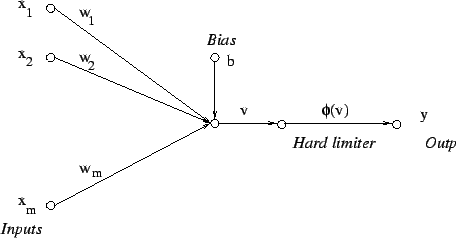
Figure 1: The signal-flow graph of the perceptron.