Tik-61.246 Digital Signal Processing and Filtering (DISKO)
Solutions, exercise round 6.
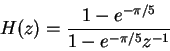
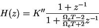
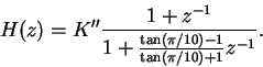
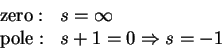
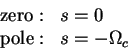
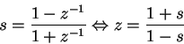
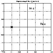
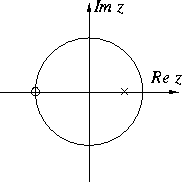
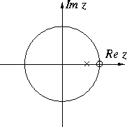
(H(z) is an anti-causal FIR,
![]() .
.
H(z) is a lowpass filter (anti-causal moving average filter).
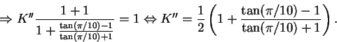
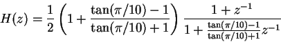
Maximum value of lowpass filter is reached
at
![]() .
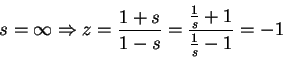
Because
.
Because
![]() ,
we get z=1 (see figure 1).
,
we get z=1 (see figure 1).
![]()
![]()
|
[Pole-zero diagram]
![\includegraphics[width=0.4\textwidth]{harj8_t1a.eps}](img15.gif) [Frequency response of H(z) with K=0.2]
[Frequency response of H(z) with K=0.2]
![\includegraphics[width=0.4\textwidth]{harj8_t1b.eps}](img16.gif)
|
In the impulse-invariant method the target is to get impulse
response of digital filter h[n] to be the same as the
sampled impulse response of analog filter ha(nT). Because IIR
filters have normally an impulse response of infinite length,
this method brings distortion.
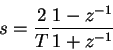
In the bilinear transform the whole left subspace of s-plane
is mapped into unit circle of z-plane. This is done by substituting
variables (see 2b).
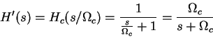
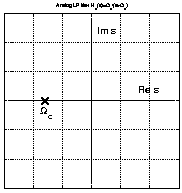
The definition of the first order (N=1) analog Butterworth filter is (Sec. 5.3.2, Eq. 5.29)
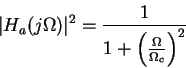
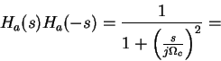
where ![]()
The pole is
![]() refers frequency in analog domain (
refers frequency in analog domain (
![]() )
and
)
and ![]() frequency in digital domain (
frequency in digital domain (
![]() ).
).
Keeping in mind that
![]() and
and
![]() ,
we get
,
we get
By inserting the values of fs=1 kHz (sampling frequency) and fc=100 Hz (cut-off frequency), we get
The transfer function is then scaled by a factor K so that the maximum
of the magnitude response will be one. We also know that the maximum is
located at zero frequency, because the frequency response of a
Butterworth filter is monotonic. Thus we get
|
[linear scale 0..1]
![\includegraphics[width=0.45\textwidth]{t2_ii.eps}](img39.gif) [desibels]
[desibels]
![\includegraphics[width=0.45\textwidth]{t2_ii2.eps}](img40.gif)
|
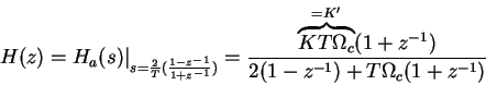
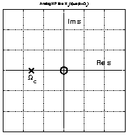
is inserted into system function (Eqs. 7.47)
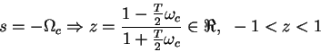
For an analog filter, the cutoff frequency must then be altered to
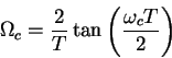
where
![]() rad/s is the desired cutoff angular
frequency.
The warped angular frequency
rad/s is the desired cutoff angular
frequency.
The warped angular frequency
![]() rad/s
is used in analog filter (see Figs. 7.7, 7.8 in Mitra).
Along with the scaling coefficient K, the transfer function of the
filter will be
rad/s
is used in analog filter (see Figs. 7.7, 7.8 in Mitra).
Along with the scaling coefficient K, the transfer function of the
filter will be
All constants (related to scaling of filter to unity) can be combined, and constants grouped in function of z
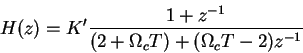
Because
![]() is constant, we can write
is constant, we can write
Now the transfer function is in standart form.
By inserting
![]() ,
we get
,
we get
As earlier, the maximum of the magnitude response is at zero frequency
Thus, the frequency response will be (figure 3)
|
[linear scale 0..1]
![\includegraphics[width=0.45\textwidth]{t2_bm.eps}](img54.gif) [desibels]
[desibels]
![\includegraphics[width=0.45\textwidth]{t2_bm2.eps}](img55.gif)
|
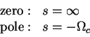
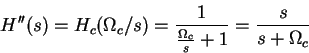
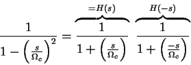
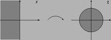
is a mapping from Laplace plane s to z-plane (figure 7)
so that
The zero of
![]() is
is ![]() and pole s=-1.
and pole s=-1.
The digital filters acquired by applying bilinear transform :
pole (omegac will not be the same as ![]() ,
use warping)
,
use warping)
Show that the best finite-length approximation to the ideal infinite length impulse response in the mean square error sense is obtained by truncated Fourier series method.
Let the
![]() denote the desired frequency response
function. Since
denote the desired frequency response
function. Since
![]() is a periodic function of
is a periodic function of ![]() with the period
with the period ![]() ,
it can be expressed as a Fourier series:
,
it can be expressed as a Fourier series:
![\begin{displaymath}H_d(e^{j\omega}) =\sum^\infty_{n=-\infty}h_d[n]e^{-j\omega n},\end{displaymath}](img81.gif)
![\begin{displaymath}h_d[n]=\frac{1}{2\pi}\int^\pi_{-\pi} H_d(e^{j\omega})e^{j\omega
n}d\omega,\ \ -\infty\leq n\leq\infty.\end{displaymath}](img82.gif)
For most practical solutions, hd is of infinite length and
noncausal. Therefore we try to find a finite-duration impulse response
sequence ht[n] of length 2M+1, whose DTFT
![]() approximates the
approximates the
![]() in some sense. One commonly used
approximation criteria is to minimize the integral squared-error
in some sense. One commonly used
approximation criteria is to minimize the integral squared-error
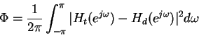
![\begin{displaymath}H_t(e^{j\omega})=\sum^M_{n=-M}h_t[n]e^{-j\omega n}.\end{displaymath}](img85.gif)
Using Parseval's relation
![\begin{displaymath}\sum_{n=-\infty}^\infty
g[n]h^*[n]=\frac{1}{2\pi}\int^\pi_{-\pi}G(e^{j\omega})H^*(e^{j\omega})d\omega,\end{displaymath}](img86.gif)
![\begin{displaymath}\Phi=\sum_{-\infty}^{\infty}\vert h_t[n]-h_d[n]\vert^2=\sum^M...
...+\sum^{-M-1}_{n=-\infty}h_d^2[n]+\sum_{n=M+1}^{\infty}h_d^2[n].\end{displaymath}](img87.gif)
It obvious from the latter form that the integral-squared error is a
minimum when
ht[n]=hd[n], for
![]() ,
that is the best
finite-length approximation to the ideal infinite-length impulse
response in the mean-square error sense is obtained by truncation.
,
that is the best
finite-length approximation to the ideal infinite-length impulse
response in the mean-square error sense is obtained by truncation.
The causality is achieved by delaying the ht[n] by M samples.
What is the disadvantage of this method and what are the solutions to this problem?
Disadvantage is the oscillatory behaviour of
![]() (Gibbs
phenomenon). This is caused by simple truncation (window function
with abrupt transitions in time domain) and the instability of the
ideal filter. Possible solutions are the use of tapered windows (fixed
or adjustable) and specification of FIRs with smooth transitions.
(Gibbs
phenomenon). This is caused by simple truncation (window function
with abrupt transitions in time domain) and the instability of the
ideal filter. Possible solutions are the use of tapered windows (fixed
or adjustable) and specification of FIRs with smooth transitions.
Some examples of window functions:
There are three figures for each item. Top left figure is the window function in time domain w[n]. The causal version can be obtained by shifting.
Bottom left figure is the window function in frequency domain
![]() .
.
The third figure in right is the amplitude frequency of actual filter which is obtained via window function method. The desired lowpass filter has normalized cut-off frequency at 0.2.
Notice that
![\begin{picture}(5623,1866)(0,-10)
\put(262,1689){\makebox(0,0)[b]{\smash{{{\SetF...
...39)
\path(3262,1839)(4162,1839)(4162,1239)
(3262,1239)(3262,1839)
\end{picture}](img98.gif)
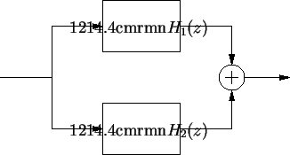
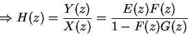
Using the flow diagram, we get the following equations:
![\begin{displaymath}\left\{
\begin{array}{ll}
Y(z) & = F(z)[X(z)E(z) + W(z)] \\
W(z) & = G(z)Y(z) \\
\end{array}
\right.
\end{displaymath}](img99.gif)
![\begin{displaymath}\begin{array}{ll}
\Leftrightarrow & Y(z) = F(z)[X(z)E(z) + G(...
...Y(z) = X(z) \frac{F(z)E(z)}{1 -
F(z)G(z)} \\ [4mm]
\end{array}\end{displaymath}](img100.gif)
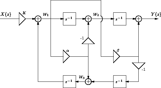
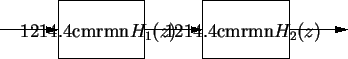
From the above figure we get the following expressions:
| W1 | = | KX+z-1W3 | (1) |
| W2 | = | (2) | |
| W3 | = | (3) | |
| Y | = | (4) |
Substituting the equation (3) in (1) we get
| (5) |
| (6) |
Next, substituting (2) in (4) we get
| (7) |
Then, from (6) and (7) we finally arrive at
 |
(8) |
Therefore
![]() for all values of
for all values of ![]() and hence
and hence
![]() if K=1.
if K=1.
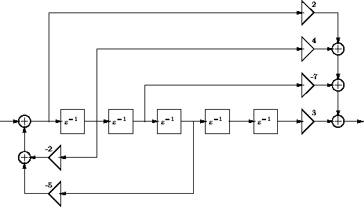
Its transposed realization:
[h]
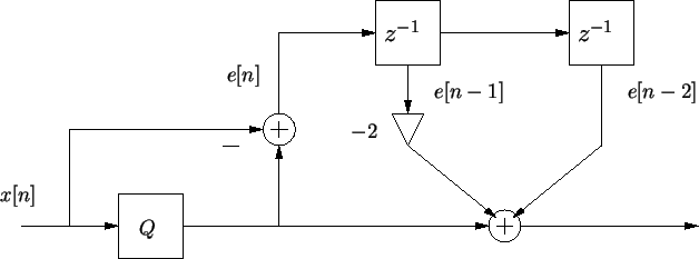
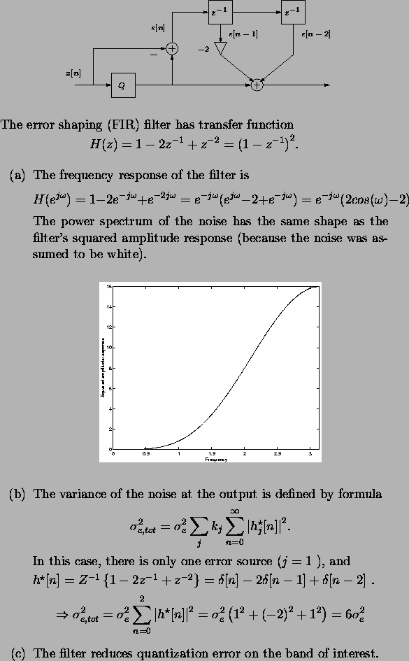
The error shaping (FIR) filter has transfer function
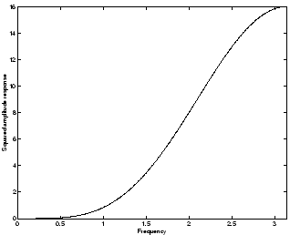
The frequency response of the filter is
The power spectrum of the noise has the same shape as the filter's squared amplitude response (because the noise was assumed to be white).
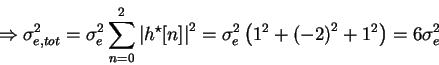
![\begin{displaymath}\sigma^2_{e,tot} = \sigma^2_e \sum_j k_j \sum_{n=0}^{\infty}
{\vert h^{\star}_j[n]\vert}^2. \end{displaymath}](img118.gif)
In this case, there is only one error source (j=1), and
![]() .
.
![\includegraphics[width=0.45\textwidth]{t4_fir_rectangular_11.eps}](img90.gif) [
[
![\includegraphics[width=0.45\textwidth]{t4_fir_rectangular_w1.eps}](img91.gif)
![\includegraphics[width=0.45\textwidth]{t4_fir_rectangular_65.eps}](img92.gif) [
[
![\includegraphics[width=0.45\textwidth]{t4_fir_rectangular_w2.eps}](img93.gif)
![\includegraphics[width=0.45\textwidth]{t4_fir_hamming_65.eps}](img94.gif) [
[
![\includegraphics[width=0.45\textwidth]{t4_fir_rectangular_w3.eps}](img95.gif)