Temporal (and linear) DSS

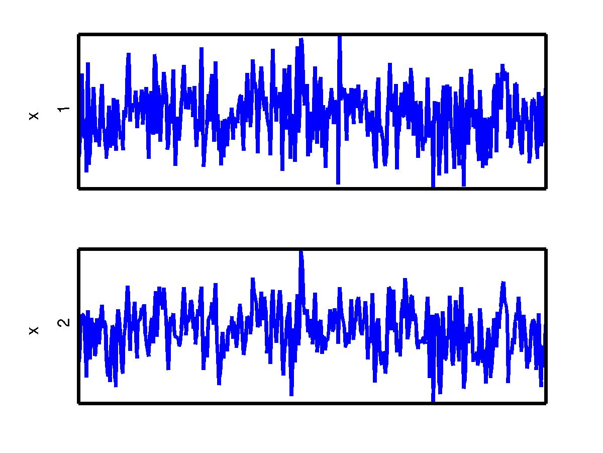
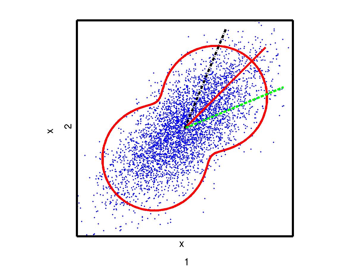
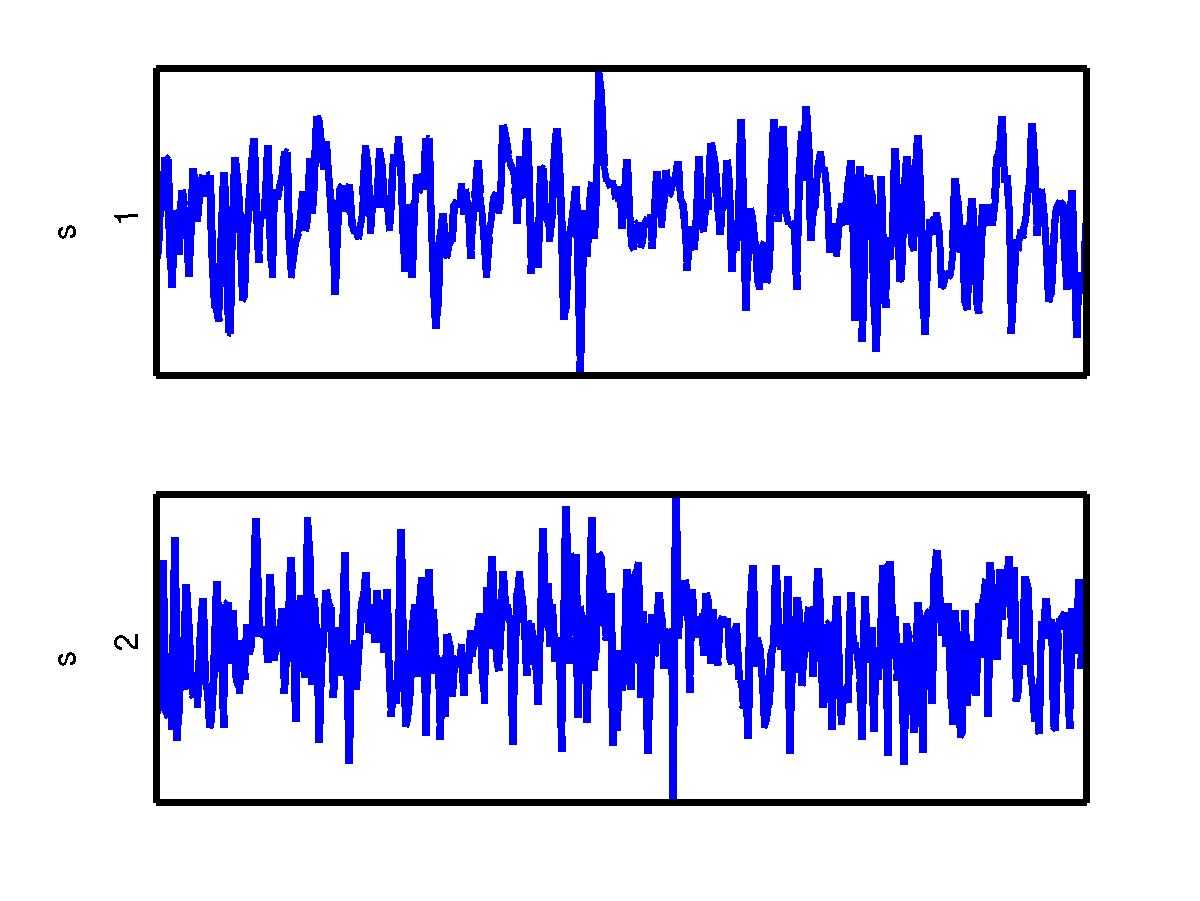
Assume two independent sources have been observed in two signals, pictured below. The left figure pictures their time course. The right figure is a scatter-plot where, at each time point, the data is represented as a point in x₁-x₂-coordinates. The green line shows the mixing coefficients of the first signal and the black line of the second signal. Red line shows the projection direction where the standard deviation of the data is maximised. Standard deviation of different projection angles have been depicted by the red nut-shaped curve.

Observed signals	Scatter plot

The aim is to recover the original signals when the true mixing is unknown.

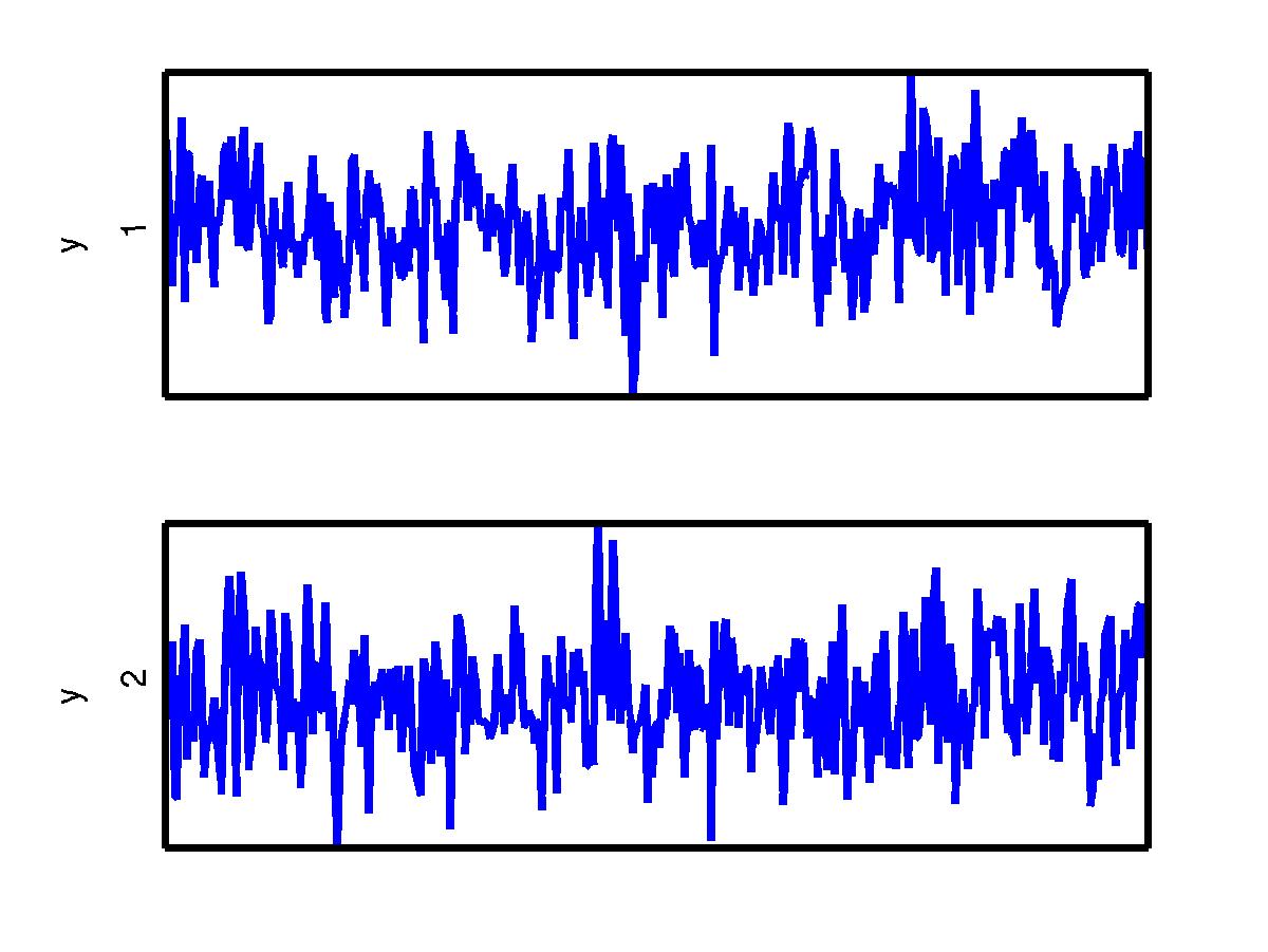
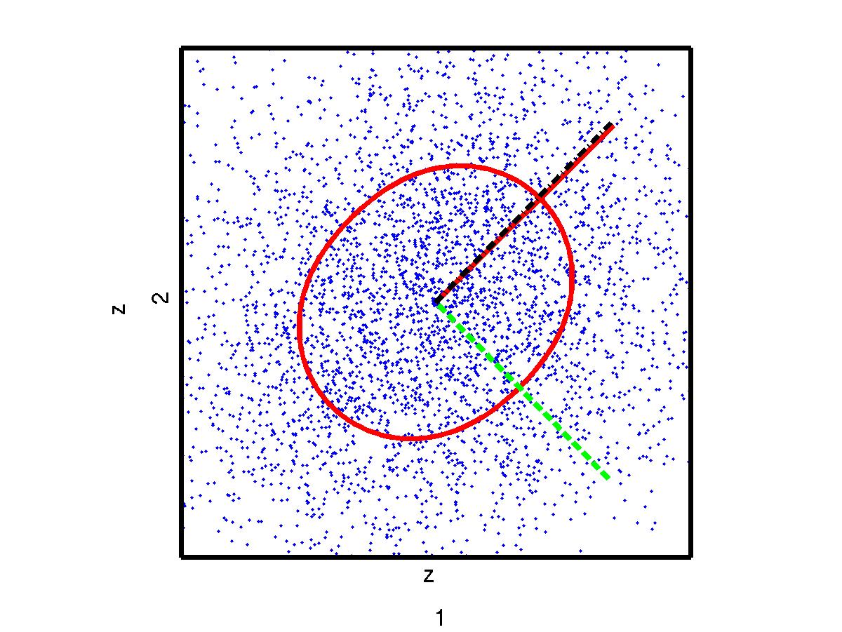
The scatter plot makes it clearly visible that the observed signals are correlated. An attempt to recover the original sources may be to seek projections that would render the signals uncorrelated. This can be done by principal component analysis (PCA). The first principal component corresponds to the most variating direction in the data (depicted in red line). In case of 2-dimensional data, the second component is the minor component and corresponds to the least variating direction. If the data is projected in the principal and minor components and their variances are normalised to unity, the resulting components are uncorrelated and have unit variance. Those components are called sphered (or whitened). They are pictured below.

Sphered signals	Scatter plot

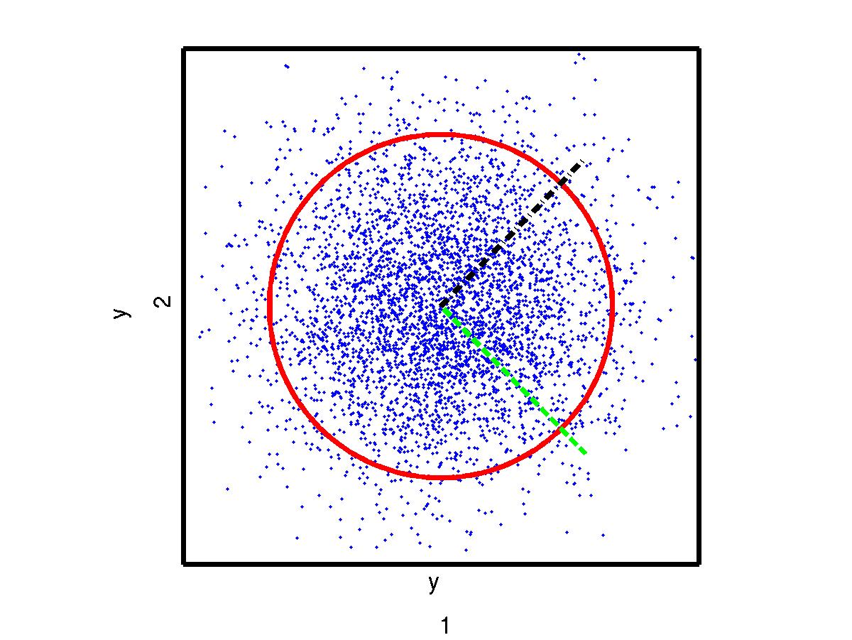Now the components y₁ and y₂ are uncorrelated. Furthermore, any direction has unit variance. This is illustrated in the fact that the standard deviation in any direction is the same. But the directions of the original sources (green and black lines) do not yet align with the sphered components.

What to do next? How to find the correct rotation to identify the sources?

Sphering has the property that all orthogonal projections result in uncorrelated components. A common name for all uncorrelated projections is factor analysis (FA). If the original sources have Gaussian distributions and the samples are independent and identically distributed (i.i.d.), FA has a rotational ambiguity and nothing more can be done. If not, any of these non-regularities may be used for separating the sources.

Now, let's see. Do the sphered components have Gaussian distributions?

Looks quite Gaussian. No luck there, too bad. But do the samples look i.i.d.? The mean and the variance seem to be quite stable. But the nearby samples seem to be correlated. To check this, let's look at a scatter plot where the coordinate pair is made from the consecutive samples.

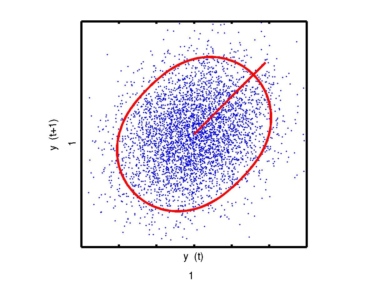
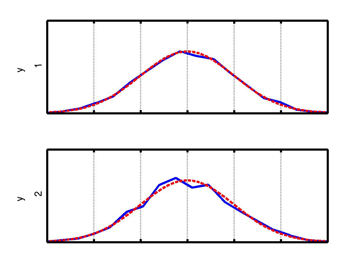
The consecutive samples are clearly correlated. Could there be a source that has significant positive correlation between nearby samples? That would mean a slowly-moving source. How to have a better estimate of it? How about denoising the whitened components? For denoising, let's just sum together the consecutive values. How does the data look then?

Voilá, the principal direction of the denoised data aligns with the first signal direction and we can identify it there. The second source may be identified with the projection orthogonal to the first one. In the figure below, the estimated signals are pictured on the left and their frequency content on the right.

Sphered signals	Scatter plot

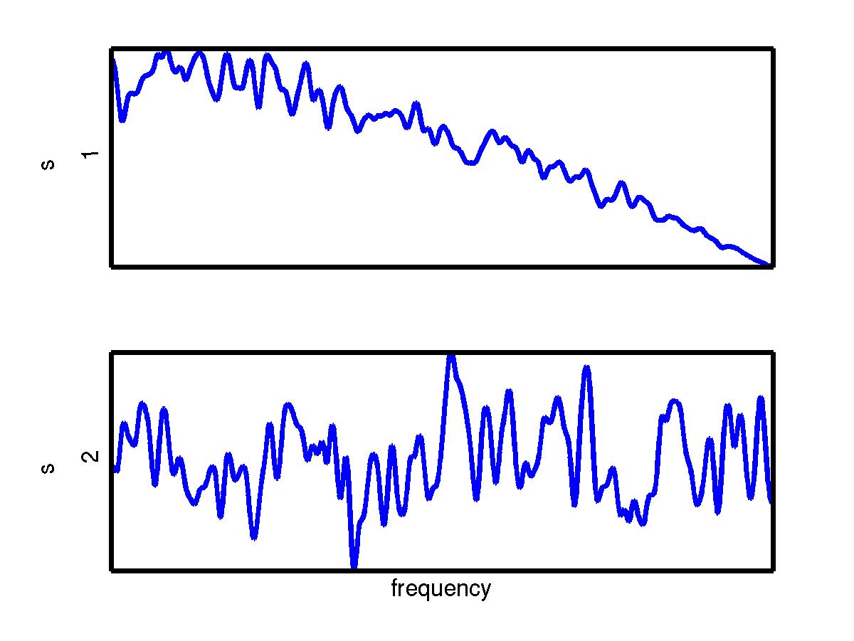The first signal seems to be a slowly-moving source, while the second an i.i.d. Gaussian.

Wow, what happened? Give me some math behind it!