The Bayes rule was formulated by
reverend Thomas Bayes in the 18th century (Bayes, 1958).
It can be derived from very basic axioms (Cox, 1946).
The Bayes rule tells how to update ones beliefs when receiving new
information. In the following,
 stands for the assumed model,
 stands for
observation (or data), and
stands for
observation (or data), and
 stands for unknown
variables.
stands for unknown
variables.
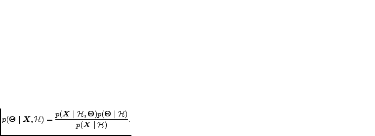
 is the prior distribution, or the
distribution of the unknown variables before making the observation. The
posterior distribution is
is the prior distribution, or the
distribution of the unknown variables before making the observation. The
posterior distribution is
 is called the likelihood of the
unknown variables given the data and the term
is called the likelihood of the
unknown variables given the data and the term
 is called the
evidence (or marginal likelihood) of the model.
is called the
evidence (or marginal likelihood) of the model.
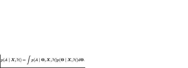
The marginalisation principle specifies how a learning system can
predict or generalise. The probability of observing  with prior
knowledge of
with prior
knowledge of
 is
is
can be acquired by
summing or integrating over all different explanations
. The term
 is the probability of given a particular
explanation
and it is weighted with the probability of the
explanation
is the probability of given a particular
explanation
and it is weighted with the probability of the
explanation
 .
.
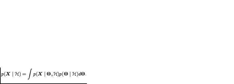
Using the marginalisation principle, the evidence term can be written as