


Next: Dirichlet distribution
Up: Standard probability distributions
Previous: Standard probability distributions
Contents
The normal distribution, which is also known as the Gaussian
distribution, is ubiquitous in statistics. The averages of
identically distributed random variables are approximately normally
distributed by the central limit theorem, regardless of their original
distribution[16]. This section concentrates on the
univariate normal distribution, as the general multivariate
distribution is not needed in this thesis.
The probability density of the normal distribution is given by
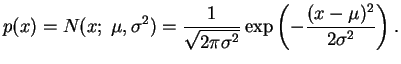 |
(A.1) |
The parameters of the distribution directly yield the mean and the
variance of the distribution:
![$ \operatorname{E}[ x ] = \mu$](img489.gif) ,
,
![$ \operatorname{Var}[ x ] =
\sigma^2$](img490.gif) .
.
The multivariate case is very similar:
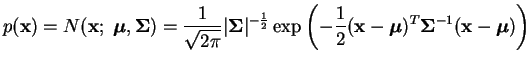 |
(A.2) |
where
 is the mean vector and
 the
covariance matrix of the distribution. For our purposes it is
sufficient to note that when the covariance matrix
is
diagonal, the multivariate normal distribution reduces to a product of
independent univariate normal distributions.
the
covariance matrix of the distribution. For our purposes it is
sufficient to note that when the covariance matrix
is
diagonal, the multivariate normal distribution reduces to a product of
independent univariate normal distributions.
By the definition of the variance
![\begin{displaymath}\begin{split}\sigma^2 &= \operatorname{Var}[ x ] = \operatorn...
...{E}[ x ] + \mu^2 = \operatorname{E}[ x^2 ] - \mu^2. \end{split}\end{displaymath}](img494.gif) |
(A.3) |
This gives
![$\displaystyle \operatorname{E}[ x^2 ] = \mu^2 + \sigma^2.$](img495.gif) |
(A.4) |
The negative differential entropy of the normal distribution can be
evaluated simply as
![$\displaystyle \operatorname{E}[ \log p(x) ] = -\frac{1}{2} \log(2 \pi \sigma^2)...
...[ \frac{(x-\mu)^2}{\sigma^2} \right] = -\frac{1}{2} (\log(2 \pi \sigma^2) + 1).$](img496.gif) |
(A.5) |
Another important expectation for our purposes
is [35]
![\begin{displaymath}\begin{split}\operatorname{E}[ \exp(-2 x) ] &= \int \frac{1}{...
...ght) dx \\ &= \exp\left(2 \sigma^2 - 2 \mu \right). \end{split}\end{displaymath}](img497.gif) |
(A.6) |
A plot of the probability density function of the normal distribution
is shown in Figure A.1.
Figure A.1:
Plot of the probability density function of the
unit variance zero mean normal distribution  .
.
|
|
Next: Dirichlet distribution
Up: Standard probability distributions
Previous: Standard probability distributions
Contents
Antti Honkela
2001-05-30
![\includegraphics[width=.5\textwidth]{pics/gauss}](img498.gif)