Tik-61.261 Principles of Neural Computing
Raivio, Venna
Exercise 6 4.3.2001
- Construct a MLP network which is able to separate the two classes
illustrated in Figure 1. Use two neurons both in the input and output
layer and an arbitrary number of hidden layer neurons. The output of
the network should be vector
![$ [1,0]^T$](img3.png) if the input vector belongs to
class
if the input vector belongs to
class
 and
and ![$ [0,1]^T$](img5.png) if it belongs to class
if it belongs to class
 . Use nonlinear activation functions, namely
McCulloch-Pitts model, for all the neurons and determine their weights
by hand without using any specific learning
algorithm.
. Use nonlinear activation functions, namely
McCulloch-Pitts model, for all the neurons and determine their weights
by hand without using any specific learning
algorithm.
- What is the minimum amount of
neurons in the hidden layer required for a perfect separation of the classes?
- What is the maximum amount of neurons in the hidden layer?
- The function
is approximated with a neural network. The activation
functions of all the neurons are linear functions of the input signals
and a constant bias term. The number neurons and the network
architecture can be chosen freely. The approximation performance of the network
is measured with the following error function:
where
 is the input vector of the network and
 is the
corresponding response.
is the
corresponding response.
- Construct a single-layer network which
minimizes the error function.
- Does the approximation
performance of the network improve if additional hidden layers are included?
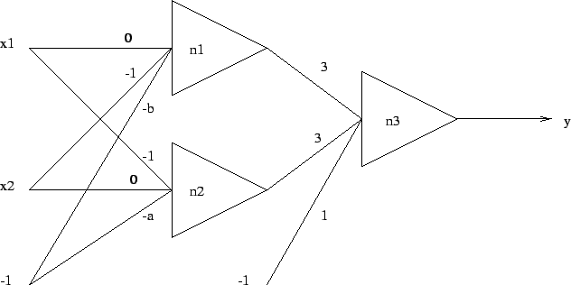
- The MLP network of Figure 2 is trained for
classifying two-dimensional input vectors into two separate
classes. Draw the corresponding class boundaries in
the
 -plane assuming that the activation function
of the neurons is (a) sign, and (b) tanh.
-plane assuming that the activation function
of the neurons is (a) sign, and (b) tanh.
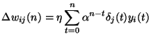
- Show that (a)
is the solution of the
following difference equation:
where  is a
positive momentum constant. (b) Justify the claims 1-3 made on the
effects of the momentum term in Haykin pp. 170-171.
is a
positive momentum constant. (b) Justify the claims 1-3 made on the
effects of the momentum term in Haykin pp. 170-171.
- Consider the simple example of a network involving a single
weight, for which the cost function is
where  ,
,  , and
, and
 are constants. A back-propagation algorithm with momentum is
used to minimize
are constants. A back-propagation algorithm with momentum is
used to minimize
 . Explore the way in which the inclusion
of the momentum constant influences the learning process,
with particular reference to the number of epochs required for
convergence versus .
. Explore the way in which the inclusion
of the momentum constant influences the learning process,
with particular reference to the number of epochs required for
convergence versus .
Figure 2:
The MLP network.
 |
Jarkko Venna
2004-03-02
![$\displaystyle \mathcal{E} = {\int}_1^2 [t(\mathbf{x})-y(\mathbf{x})]^2 d\mathbf{x},$](img9.png)
![\begin{figure}%%[h]
\centering\epsfig{file=mlp_classification.ps,width=100mm}\end{figure}](img21.png)