Project work

The project work involves semantic image classification based on a set of precomputed low-level features. The selection of the used classification algorithm is free, but the provided examples apply support vector machines using the LIBSVM implementation. The deadline for the project work is May 19th, 2008.

We use the image data from The PASCAL Visual Object Classes Challenge 2005, datasets 1 and 2. The data sets contain a total of 2329 images of motorbikes, bicycles, people, and cars in arbitrary pose. The set is divided into a training set of 684 images, and two test sets containing 689 and 956 images, respectively. You may download the original images from the challenge website for reference, although it is possible to do the project work entirely based on the provided low-level features.

The set of pre-computed low-level features are:

The feature data can be found here in LIBSVM format (6.8 MB). The classwise ground truth for test set 2 is also available (4.4 MB). See the LIBSVM README file for a description of the format.

The file names of the images in correct order are given in the files trainset and testset1 for the training set and test set 1, respectively. The file testset2 contains the image labels given for the randomized test set 2.

For more details about the features, see the MPEG-7 overview and this ICCV 2003 paper by Gy. Dorkó and C. Schmid.

The task is to train classifiers for the four concepts (motorbikes, bicycles, people, and cars) using the training set and then test the classifiers using the test sets. The examples shown in this section use the command-line version of LIBSVM, but you are free to use any other implementation or algorithm. In particular, there is a Matlab interface for LIBSVM available if you prefer to use Matlab. Also, you can use the included read_sparse function to read in LIBSVM format data files to Matlab and then use some other algorithm for the classification.

An example SVM classifier

In the following, we assume that you have downloaded (and compiled) LIBSVM, and have all the low-level feature files in a subdirectory voc2005 of the LIBSVM main directory. We assume here that you are using some variant of Unix/Linux that has Python and Gnuplot installed. Windows binaries for LIBSVM can be found in the windows subdirectory.

First, let us scale the training and test sets into the range [-1,1]:

$ cd voc2005
$ ../svm-scale -l -1 -u 1 -s EdgeHistogram-bicycles.train.range EdgeHistogram-bicycles.train > EdgeHistogram-bicycles.train.scale
$ ../svm-scale -r EdgeHistogram-bicycles.train.range EdgeHistogram-bicycles.test1 > EdgeHistogram-bicycles.test1.scale

LIBSVM provides a tool for SVM parameter estimation using grid search and cross-validation:

$ ../tools/grid.py EdgeHistogram-bicycles.train.scale

which outputs the best values it found for C and gamma. You may now focus the grid search to the neighborhood of the best values with options -log2c and -log2g.

Once we have the parameter values, we are ready to train the SVM classifier:

$ ../svm-train -c C -g gamma -b 1 EdgeHistogram-bicycles.train.scale EdgeHistogram-bicycles.train.model

where C and gamma are the values found by grid.py. The option -b 1 is needed to get the probability estimates for the test images.

The classifier is tested using the images in the test set 1:

$ ../svm-predict -b 1 EdgeHistogram-bicycles.test1.scale EdgeHistogram-bicycles.train.model EdgeHistogram-bicycles.test1.output

which prints out the overall accuracy and the individual probability estimates for the test images in EdgeHistogram-bicycles.test1.output.

Fundamentals

Train models for all four concepts using the given features. Report the results of test set 1 with the concept-wise and overall classification accuracy and average precision (see Chapter 13 in the course book). You may also use some other suitable information retrieval measures such as recall-precision curves or receiver operating characteristic (ROC) curves. For these measures, you need to look at the individual probability estimates in the .output files and sort the test set images accordingly.

For test set 2, return an ordered list of the images for each concept as separate text files, one image per line. The lists should contain the images that your method finds most probable for being relevant to the given concept, in decreasing order. The lists may or may not contain all 956 images, but the performance may suffer if you return only partial lists. We will then calculate the mean average precision for all submitted experiments and publish the results on the course web page. Submit the lists for only your best method or methods to Mats Sjöberg (mats.sjoberg (at) tkk.fi) before April, 21st, 2008.

Improvements

There are a number of ways you can extend your experiments:

• The lack of positive examples. Adjust the classifier due to the greater number of negative examples, e.g. by removing some negative images from the training data or using the -w-1 option (see LIBSVM documentation).
• Early fusion. Concatenate multiple features together before training the SVMs.
• Late fusion. Combine results from multiple features together using a suitable function for the probability estimates or the retrieval ranks of the images.
• Fault analysis. Look at the original images and try to analyse why certain images are classified incorrectly.
• Four-class classification. Classify each test image into only the most probable class and compare the results.
• Try other SVM kernels instead of the default RBF kernel.
• Try other classification algorithms.
• Something else.

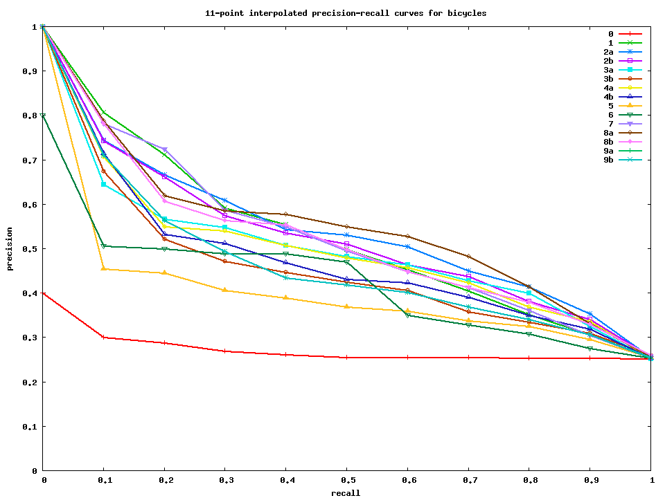
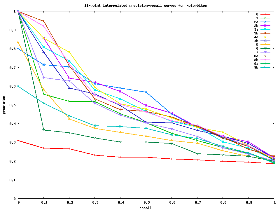
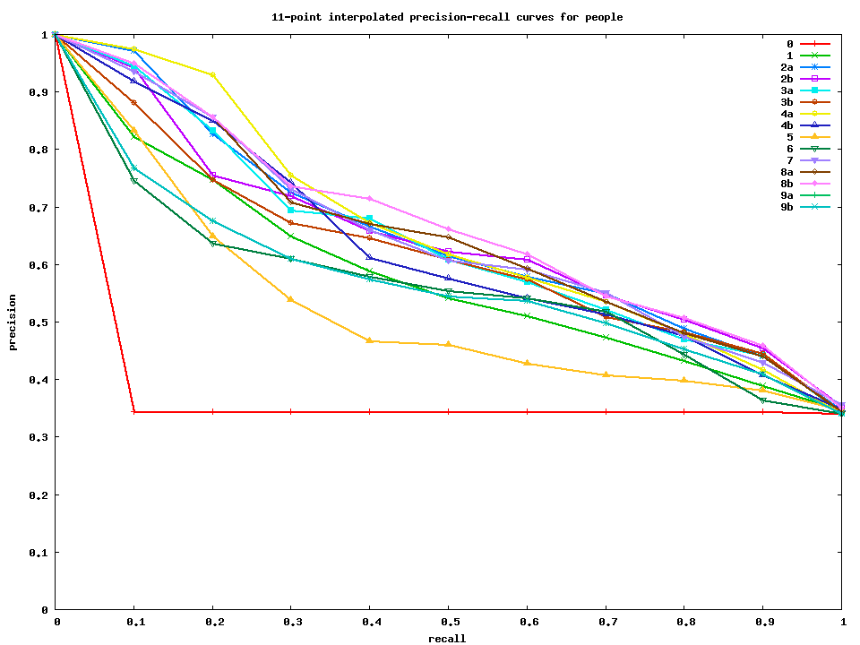
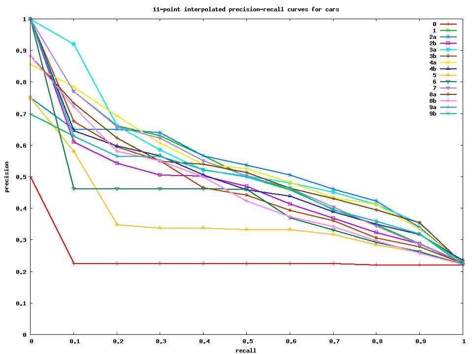
Select and include at least two items from the list to your project.

Test set 2 results

The average precision results for submitted test set 2 runs are as follows:

Interpolated precision-recall curves for bicycles, motorbikes, people, and cars. Gnuplot and data files for making these curves are also available.

The results of the project work should be reported in a scientific conference style paper, which should be understandable as such, i.e. without these instructions, and complete with a title, abstract, introduction, methods, results and discussion sections, and references.

Send the final report in PDF format to Mats Sjöberg (mats.sjoberg (at) tkk.fi). The deadline for the project work is May 19th, 2008. The report can be written in English, Finnish, or Swedish.