T-61.5020 Statistical Natural Language Processing
Answers 9 -- Statistical machine translation
Version 1.1
- 1.
- We are trying to find the most probable translation
 for the
Swedish sentence
for the
Swedish sentence  :
:
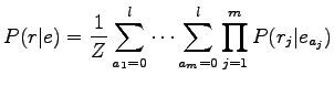
Let's use the model presented in the course book for the probability
 :
:
where  is the lenght of the original Swedish sentence and
  is the
lenght of the translated English sentence. For the two possibilities:
is the
lenght of the translated English sentence. For the two possibilities:
Here we tried the all possible translation rules for each Swedish
word. Because the set of the rules is very sparse, the calculation
became as simple as that.
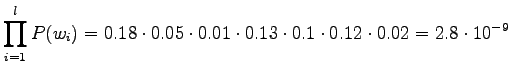
The prior probablity  is obtained from the language model.
Let's calculate it for both of the models:
is obtained from the language model.
Let's calculate it for both of the models:
By multiplying the prior and the translation probability, we see that
the latter translation is more probable:
Notice that our translation model does not care about the word
order. As neither the unigram model does that, the full model gives
no importance to the order. Also, if the most probable sentence is
asked instead of testing alternatives, there will be no articles or
word ``into'' in it. The reason is that adding them will not affect
the translation probability, and always reduces the language model
probability. So the language model favours shorter sentences. By
increasing the model context to trigram we might get a model that
puts the articles and word order better in their place.
In common case we need some heuristics to choose the translations that
will be considered. Calculating probabilities for all the possible
alternatives is impossible in practice.
- 2.
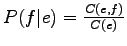
- Let's use the word
 = ``tosiasia'' (fact) as an example. It has
occurred in 983 sentences. In order to do normalization, we must also
count the number of occurrences (sentences where they occurred in) for
every English word.
= ``tosiasia'' (fact) as an example. It has
occurred in 983 sentences. In order to do normalization, we must also
count the number of occurrences (sentences where they occurred in) for
every English word.
Twenty English words that had the largest values for the number of
co-occurrences and the normalized number of co-occurrences are
given in the table below. We see that neither of the methods gave
desired results. For unnormalized frequencies, the problem is with the
very common words, that occur in almost any sentence and thus also
with our . For normalized frequencies, the problem is reversed,
i.e. very rare words. If a word that occurs only once happen to occur
with , it will give the maximum value,  .
.
 |
 |
| the |
851 |
| that |
765 |
| is |
720 |
| fact |
632 |
| of |
599 |
| a |
523 |
| and |
515 |
| to |
497 |
| in |
481 |
| it |
318 |
| this |
311 |
| are |
246 |
| we |
243 |
| not |
239 |
| for |
221 |
| have |
210 |
| be |
199 |
| which |
192 |
| on |
182 |
| has |
173 |
|
|
 |
| winkler |
1.0000 |
| visarequired |
1.0000 |
| visaexempt |
1.0000 |
| veiling |
1.0000 |
| valuejudgment |
1.0000 |
| undisputable |
1.0000 |
| stayers |
1.0000 |
| semipermeable |
1.0000 |
| rulingout |
1.0000 |
| roentgen |
1.0000 |
| residuarity |
1.0000 |
| regionallevel |
1.0000 |
| redhaired |
1.0000 |
| poorlyfounded |
1.0000 |
| philippic |
1.0000 |
| pemelin |
1.0000 |
| paiania |
1.0000 |
| overcultivation |
1.0000 |
| outturns |
1.0000 |
| onesixth |
1.0000 |
|
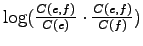
The problem in the previous methods was that they did not take into
account the bidirectionality of the translation: For to be a
probable translation for , should occur in those sentences
were occurred, and also should occur in those sentences were
occurred. In this case, both probability estimates
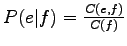 and
and
 should be high. Let's use the product of those probabilities as the
weight for .
should be high. Let's use the product of those probabilities as the
weight for .
The results are in the left-most table on the next page. This time we
found the correct translation, and another closely related word,
reality, has the next highest value.
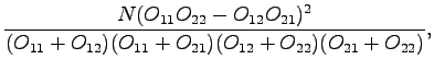
Let's try also the  test that was presented in context of
the collocations:
test that was presented in context of
the collocations:
where
and  is the number of sentences in the corpus. For the words
that will get the value over 3.843, the probability
that the co-occurrences were there by chance is less than 5%.
is the number of sentences in the corpus. For the words
that will get the value over 3.843, the probability
that the co-occurrences were there by chance is less than 5%.
The words that have the largest values are it the right-side table.
The test seems to work very nicely: Only ``fact'' exceeded the
chosen confidence value. On the other hand, if we would like to
have alternative translations, such as ``reality'', a method that
gave probability values would be more convenient.
In practice, the translation probabilities are often determined
iteratively using the EM algorithm. This way one can limit that
one English word would be a translation for many Finnish words.
However, a method such as above might be used for initialization of
the probabilities.
|
 |
| fact |
-4.0184 |
| reality |
-6.0493 |
| winkler |
-6.1975 |
| that |
-6.3200 |
| is |
-6.4256 |
| visarequired |
-6.8906 |
| visaexempt |
-6.8906 |
| veiling |
-6.8906 |
| valuejudgment |
-6.8906 |
| undisputable |
-6.8906 |
| stayers |
-6.8906 |
| semipermeable |
-6.8906 |
| rulingout |
-6.8906 |
| roentgen |
-6.8906 |
| residuarity |
-6.8906 |
| regionallevel |
-6.8906 |
| redhaired |
-6.8906 |
| poorlyfounded |
-6.8906 |
| philippic |
-6.8906 |
| pemelin |
-6.8906 |
|
|
|
| fact |
17.3120 |
| reality |
2.2027 |
| winkler |
2.0000 |
| that |
1.4287 |
| is |
1.2133 |
| visarequired |
1.0000 |
| visaexempt |
1.0000 |
| veiling |
1.0000 |
| valuejudgment |
1.0000 |
| undisputable |
1.0000 |
| stayers |
1.0000 |
| semipermeable |
1.0000 |
| rulingout |
1.0000 |
| roentgen |
1.0000 |
| residuarity |
1.0000 |
| regionallevel |
1.0000 |
| redhaired |
1.0000 |
| poorlyfounded |
1.0000 |
| philippic |
1.0000 |
| pemelin |
1.0000 |
|
svirpioj[a]cis.hut.fi