|
We can see that the estimates given by a human are somewhat adrift and statistics badly so.
Statistics were estimated from a corpus of 30 million words. In that corpus, none of the trigrams occured even once. If the words were stemmed, 11 sentences were found that had the trigram ``tuntua jo hyvä''. The estimate needs badly some smoothing, and it will not be very good even after that.
Also the estimates given by our human can be doubted, as some quite possible senteces have a probability of zero. One example might be ``Kyllä alkaa tuntumaan jo kumisaapas jalassa'' (free translation: ``Now the rubber boots are beginning to feel in my feet''), something that one might say after a long walk.
When the full sentence was given to the test person, we got quite good estimates (third column). To get even close with a computer, the language model would need understand grammatical syntax of Finnish as well as sematic meaning of words (e.g. that February is in the end of winter season).
- a)
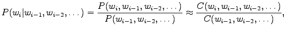
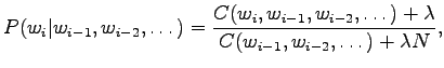
- The maximum likelihood estimates can be calculated as
where function tells the number of occurrences in the training set.
In the unigram estimates we forgot everything about the previous words, brigram estimates depend on just one previous word, and trigram estimates use a history of two words.
For unigrams
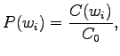
where is number of samples in the training set. These estimates
are independent of the word histories.
is number of samples in the training set. These estimates
are independent of the word histories.


In the bigram estimates we use the previous word, i.e.

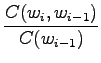


None of the word combinations that did not occur in the training data are possible for this model. - b)
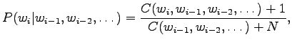
- Laplace estimation corresponds to a prior assumption that all
words have uniform probabilities. In practise, it is assumed that
each word is seen already once:
where is the size of the vocabulary.
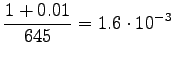
So we get the following estimates for unigrams:
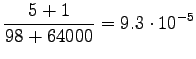
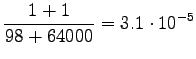
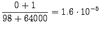
And bigrams:
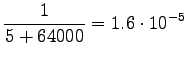
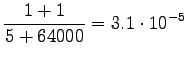

Take notice that the uniform prior affects the estimates much. All words have almost the same probability. - c)
- In Lidstone estimate we can control how much we trust in the
uniform prior. We assume that all the words are seen
 times
before the training corpus:
times
before the training corpus:
where we were asked to set . The estimates are:
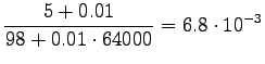

Bigrams:
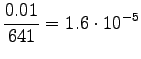
Here the training data has more clear control on the estimates. A suitable value for can be found by taking part of the
training data out of the actual training and using it to optimize
the parameter.
Here
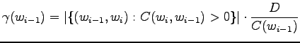 |
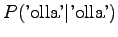
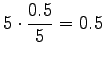
Let's start by calculating the interpolation coefficients for the
histories ``olla'' and ``vaikuttaa''. The first one had five different
right contexts (following words) and it has occurred five times.
The second one has occurred one once and thus with one right context.
 |
|||
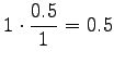 |
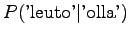
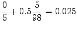
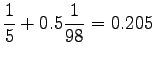
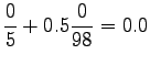
Now we can estimate the interpolated bigram probabilities:
 |
|||
 |
|||
 |
|||
 |
|||
 |
|||
 |
Notice that the method does not give any probability mass to words that did not occur in the training data, such as ``gorilla''. This can be fixed by using some additional smoothing method for the unigram. Another alternative would be to continue the interpolation with an uniform distribution (sometimes called ``zero-gram'').
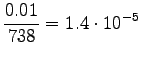
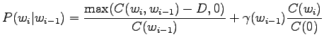
Interpolation or back-off to lower order n-grams is not always
very reliable. As an example, think about the bigram
``San Francisco''. As the name is quite commonly used, the estimate
![]() would be very reliable.
So if the previous word was ``San'', no problems there. But what if
it wasn't? In this case, the probability of ``Francisco'' should be
clearly lower than it is if we use the unigram distribution without
any idea of the previous word. Based on this idea, Kneser-Ney
smoothing estimates the lower order distributions by calculating
how many times the observed word to occurs in a new context.
The current state-of-the-art smoothing technique is modified Kneser-Ney
interpolation, that applies this kind of type counts and absolute
discounting with three separately optimized discounts.
would be very reliable.
So if the previous word was ``San'', no problems there. But what if
it wasn't? In this case, the probability of ``Francisco'' should be
clearly lower than it is if we use the unigram distribution without
any idea of the previous word. Based on this idea, Kneser-Ney
smoothing estimates the lower order distributions by calculating
how many times the observed word to occurs in a new context.
The current state-of-the-art smoothing technique is modified Kneser-Ney
interpolation, that applies this kind of type counts and absolute
discounting with three separately optimized discounts.
 |
|||
 |
|||
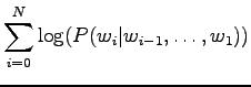
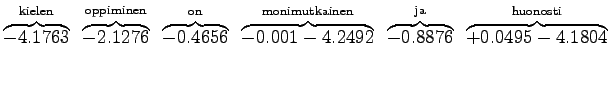
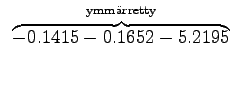
Now we can count the sum of the logarithmic probabilities:
 |
|||
 |
|||
 |
|||
For those words that had no trigram probabilities, we had to use both back-off coefficients and bigram probabilities. If neither bigram was found, we had to back-off again.
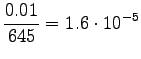
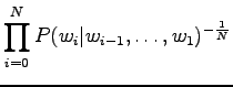
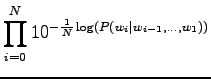
Inserting the result to the expression of perplexity:
 |
This can be thought as that the model corresponds to one that must choose between 1200 equally probable words each time. Word ``tapahtumaketju'' was not in the 64000 most common words and thus not included in the model. So the out-of-vocabulary rate for the model is