- a)
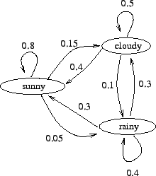
- The Markov chain is drawn in figure 1.
- b)
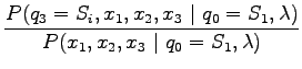
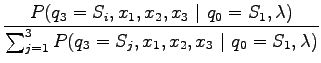
- Let's calculate the probability for state sequence
 when we know that we start
from state
when we know that we start
from state  :
:


Let's apply the Markov assumption:
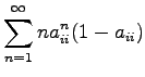
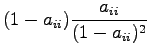
This corresponds to the coefficients
 |
|||
 |
|||
 |
|||
 |
In the case of sunny days
 |
|||
 |
Above we used first the formula
![]() .
Then we noted that
.
Then we noted that
![]() . Denominator and numerator
of the equation have similar terms. Let's lighten the notes using
the function
. Denominator and numerator
of the equation have similar terms. Let's lighten the notes using
the function
![]() :
:
 |
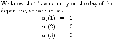
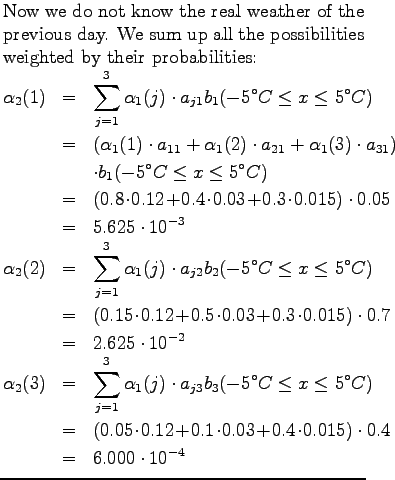
Now we will examine how this forward probability
![]() can be
calculated.
can be
calculated.
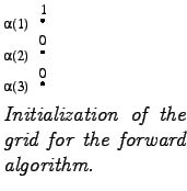
Initial day
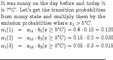
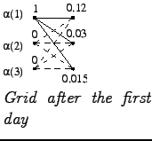
First day
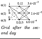
 Second day
Third day
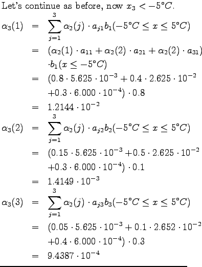
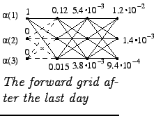
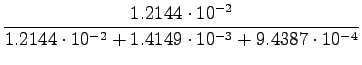
Now we have calculated all the neccessary quantities. Let's insert them
to the equation:
 |
|||
 |
|||
So the probability that it is sunny on the day of the return is 89 %. In a similar manner we can calculate the probability of a cloudy (10 %) and a rainy (1 %) day.
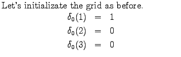
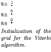
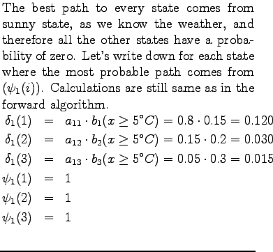
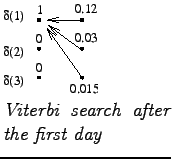
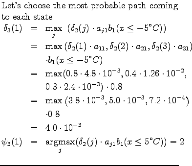
b) This time we try to guess the most probable sequence of weather. In can be done using the Viterbi algorithm, which is very similar to the forward algorithm. The difference is that in each state we now calculate the probability over the best sequence instead of summing up all the sequences. Viterbi: Initial day
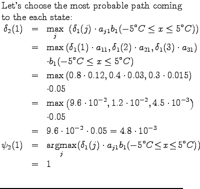
Viterbi: First day
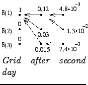
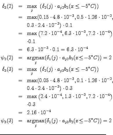
 Viterbi: Second day
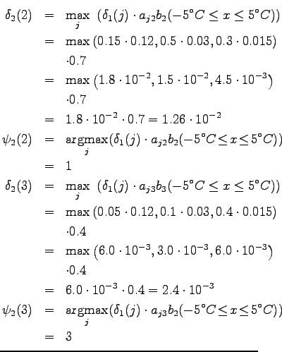
 When counting
 ![]() we note that the probabilities were same from
the states 1 and 3. We can make an arbitrary choice between them. Here
the choice was 3.
we note that the probabilities were same from
the states 1 and 3. We can make an arbitrary choice between them. Here
the choice was 3.
Viterbi: Third day
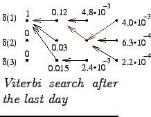 From the final grid we can get the most probable sequence of states:
Let's start from the most probable end state and follow the arrows
backwards to the beginning. It seems that it has been sunny, cloudy
and again sunny.
From the final grid we can get the most probable sequence of states:
Let's start from the most probable end state and follow the arrows
backwards to the beginning. It seems that it has been sunny, cloudy
and again sunny.
Conclusion: The differece between forward and Viterbi algorithms
The forward algorithm gives the correct probability for each state sequence. However, it cannot be used to get the most probable path from the grid.
In Viterbi search, the state probabilities are just approximations. However, it can correctly find the best path.
Computationally both of the algorithms are equally burdensome. Summing in the forward algorithm has just changed to maximization in the Viterbi algorithm.