T-61.5020 Statistical Natural Language Processing
Answers 2 -- Similarity measures
Version 1.0
- 1.
-
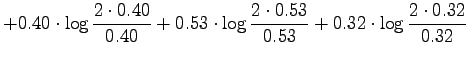
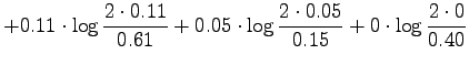
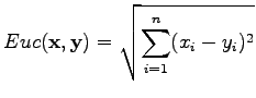
Euclidean distance between the vectors
![$ \mathbf x =[x_1 ~x_2 \dots x_n]$](img2.png) and
and
![$ \mathbf y =[y_1 ~y_2 \dots y_n]$](img3.png) is defined as
is defined as
 |
(1) |
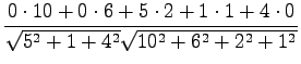
The distance between Tintus and Koskisen korvalääke is calculated as
an example:
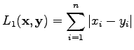
The distance according to the  norm is defined as
 |
(2) |
So the distances are:
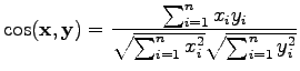
The cosine measure is a little different case. It can be defined as
 |
(3) |
Let's calculate the distances:
Here a larger value corresponds to a larger similarity, so
the distances are in the same order as before.
For the information radius we formulate the maximum likelihood estimates
for that the next word is generated by a source  (Tintus,
Korvalääke, Termiitti) is
(Tintus,
Korvalääke, Termiitti) is  . This is done by dividing the each
element of the table by the sum of its row (Table 1).
. This is done by dividing the each
element of the table by the sum of its row (Table 1).
Table 1:
ML estimates for the word probabilities
| |
fresh |
acidic |
sweet |
fruity |
soft |
| Tintus |
0 |
0 |
0.50 |
0.10 |
0.40 |
| Korvalääke |
0.53 |
0.32 |
0.11 |
0.05 |
0 |
| Termiitti |
0.07 |
0.29 |
0.21 |
0.21 |
0.21 |
|
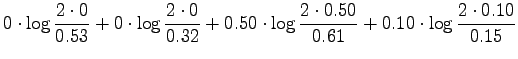
Last we define that
The information radius is given by the formula
Let's calculate it for the given sources:
We see that all the measures set the medicines to a similar order:
Tintus and Temiitti are the most similar ones, Tintus and Korvalääke
are the most different.
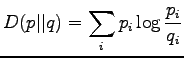
From the definition of the KL divergence we can directly see some of
its problems:
First, the KL divergence is not symmetric, so we should each time
decide which one of the two drugs is the reference drug  . The
second problem is that if the compared distribution has a zero
probability in some dimension where the reference distribution has a
non-zero probability, the divergence goes to infinity.
. The
second problem is that if the compared distribution has a zero
probability in some dimension where the reference distribution has a
non-zero probability, the divergence goes to infinity.
[2.]
The definition of the Kullback-Leibler divergence was
Let's find a distribution that minimizes the KL divergence. We add
a Lagrange coefficient  to make sure that shall be
a correct probability distribution (i.e.
to make sure that shall be
a correct probability distribution (i.e.
 ) and
) and
 for
for  .
.
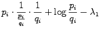
Let's set the partial derivative with respect to the  to zero:
Now we solve :
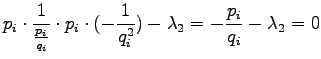
Let's calculate the partial derivative with respect to :
A similar condition is obtained for  when derivating with respect to
(which was exactly the purpose of the multipliers). The last
condition is obtained by derivating with respect to
:
when derivating with respect to
(which was exactly the purpose of the multipliers). The last
condition is obtained by derivating with respect to
:
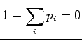
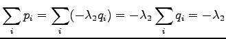
Because both and should sum up to one, we get:
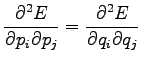
Considering the second order derivates we can make sure that this
is really the minimum and not maximum:
If we set  to the formula of KL divergence we get the
divergence of zero. So KL divergence is zero if and only if the
distributions and are equal, otherwise greater than zero.
to the formula of KL divergence we get the
divergence of zero. So KL divergence is zero if and only if the
distributions and are equal, otherwise greater than zero.
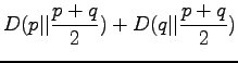
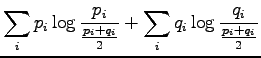
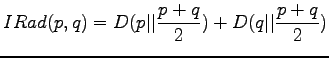
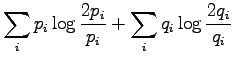
The definition of the information radius is
We just calculated that the KL divergence is zero if the distributions
are same, and larger than zero if not. In the case of the information
radius, the zero divergence is also obtained if and only if :
So the condition is the same as before.
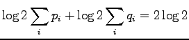
Definition of the norm is
Clearly the smallest value is zero, which comes only if .
To conclude, we notice that all the measures give zero distance with
the same condition: The distributions must be equal.
[3.]
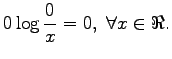
Let's look at the definition once more:
We can see that if  when
when  we get the distance
  .
.
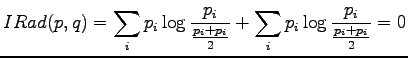
Let's write the definition of information radius open:
With intuition we might guess that a suitable distribution would be
one where the distributions are in completely separate areas:
Let's insert these to the equation:
We knew that this was the largest distance. To prove that it really
is, and that the guessed conditions are required to get it, would be
somewhat more diffcult.
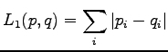
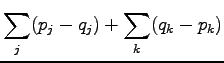
The definition for the norm was
With intuition we could say that the answer is the same as with
information radius, but let's try to prove it more mathematically.
We separate the elementary events  to two sets. In set
  were have the cases where
  and in set
  the cases
where
the cases
where  . Using these,
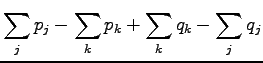
As the probabilities are positive and sum up to one, the largest
distance is get when
so the distance is
For both information radius and norm, the same conditions
for the distributions are required to get the largest distance.
The KL divergence, however, goes to infinity already when the distribution
is zero somewhere where the reference distribution is not.
svirpioj[a]cis.hut.fi