- a)
- Let's initialize the grid such that the initial state is
 .
We will collect only non-zero probability values.
.
We will collect only non-zero probability values.


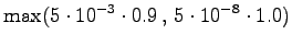
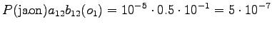
The first observation
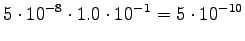
The initial state can lead only the second or fourth state, so let's calculate those probabilities:


The second observation
From the second state we can go to the third state, and from the fourth state to the fifth state, so there is no choices to be made for those steps.


However, we should notice that the states and
and  can lead to
the initial state with a null transition. Thus after the second observation
we can go also to :
can lead to
the initial state with a null transition. Thus after the second observation
we can go also to :


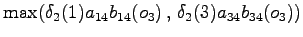
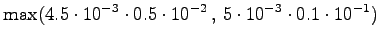
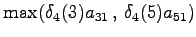
The third observation
Now the possible transitions are from
to  or
or  , and from
to .
, and from
to .


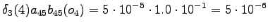
The fourth observation
Again, from
we can go only to and from to .


Final state
In the end we should arrive to the final state
. With a null
transition:

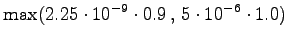


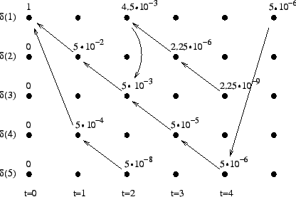
The calculated grid is in the Figure 1. By following the arrows from the end to the beginning, we obtain the most probable sequence
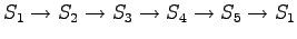 . This corresponds to the
word ``jaon''.
. This corresponds to the
word ``jaon''.
- b)
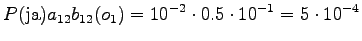
- In this case we must take into account the probabilities given by the
language model. The probability values
 are calculated
conditioned by the different choice of the word
are calculated
conditioned by the different choice of the word  :
:
 .
The probability for the word is added to the calculations at each point
where the word is selected. When we arrive to the initial state again,
the selections determine which of the bigram probabilities is used.
After that, they can be forgotten, as the language model does not
use longer contexts.
.
The probability for the word is added to the calculations at each point
where the word is selected. When we arrive to the initial state again,
the selections determine which of the bigram probabilities is used.
After that, they can be forgotten, as the language model does not
use longer contexts.
Let's initialize the grid as before. We do not select the word yet.

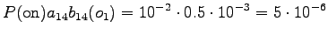
The first observation
The initial state leads to
and . The second state can
start either the word ``ja'' or ``jaon'', so both must be taken into
account.


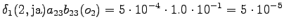
The second observation
The second state leads only to the third state and the fourth state to the fifth state. In addition, the first state can be reached with a null transition. This is of course possible only for the words that end at this point.


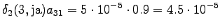


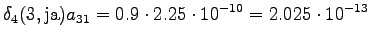
The third observation
Possible transitions are from
to or , and from to
. The transitions from start new words, so the probabilities
from the language model are taken into account. In addition, as we had
two possible words in state , we can now select the more probable one.


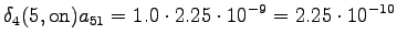
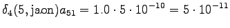
The fourth observation
From the second state we can only to the third state, and from the fourth state only to the fifth state. Also the first state can be reached with a null transition.


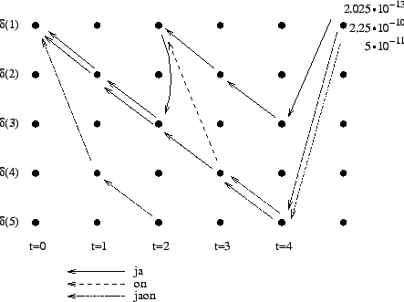
The grid after the final step is in Figure 2. The different word choices are drawn with different arrows. The most probable of the three paths that have led to the final state is
 . When we follow the arrows backwards
in time, we get the most probable sequence
. When we follow the arrows backwards
in time, we get the most probable sequence
 . This corresponds
to the two-word sequence ``ja on''.
. This corresponds
to the two-word sequence ``ja on''.
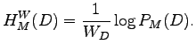
Instead of direct comparison, we can first normalize the entropies so
that they are based on words. The cross-entropy of test data ![]() could
be calculated as
could
be calculated as
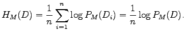
If we divide the logarithm of data likelihood
As we know
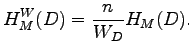
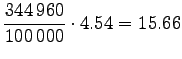
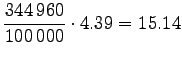
Let's convert the given entropies to word-based estimates:
 |
|||
 |
|||
 |
|||
 |
|||
 |
|||
 |
It seems that the entropies with the segmentation B are somewhat better in models of all magnitudes. However, as the differences are small, and models B have larger models, the exact sizes must be taken into account. The comparison is easy if we draw plot the results to size-entropy coordinates; see Figure 3.
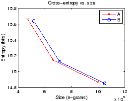
The break-line that connects the points of the segmentation A is nearer to the left-down corner that the lines of connecting B, which means better accuracies for the models of same size.
Next we will take a look at the recognition results. The error rates have been calculated per words, so there is no need for normalization. The word error rates (WER) are plotted against model sizes in Figure 4. We see that the results are mixed for the small and large models: Segmentation A works better for the small models, but B seems to outperform it after the size grows over 900000 n-grams.
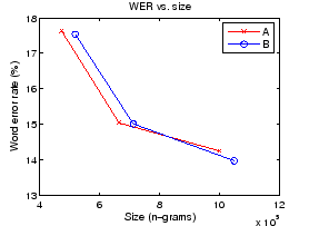
It seems to be quite clear that the models based on segmentation A are better than those based on B, if the model size is small. For larger models, the results are very close. In addition, the performance is not known for models smaller than half million or larger than one million n-grams. To get more reliable results, we would need more measurement points and test the statistical significance between the values (e.g. with Wilcoxon signed-rank test).