T-61.5020 Statistical Natural Language Processing
Answers 1 -- Basics of probability calculus
Version 1.0

1.

First of the given probabilities, $P(~\textrm{word is abbreviation} ~\vert~ \textrm{word has three letters}~) = 0.8$, tells that is we see a word of three letters, the probability that it is an abbreviation is 0.8, and 0.2 for something else. Next one, $P(~\textrm{word has three letters}~) = 0.0003$, tells that the probability for a random word being exactly three letters long is $0.0003$.

The probability for a random word being three letter abbreviation is get by product of the given probabilities. First we look how probable it is for a word to be three letters long, then how probable it is to be abbreviation when being three letters:

$$P(~\textrm{word is abbreviation},\textrm{word has three letters}~)$$

$$= P(~\textrm{word has three letters}~)\cdot P(~\textrm{word is abbreviation} ~\vert~ \textrm{word has three letters}~)$$

$$= 0.0003*0.8=0.00024$$

2.

Let's mark the stem ``se'' by $C_1$ ja stem ``siittää'' by $C_2$. The result of the recognition is $T$ and correct stem $O$. Now we can write the given probabilities:

$$P(T=C_1\vert O=C_1) = 0.95$$

$$P(T=C_1\vert O=C_2) = 0.05$$

$$P(T=C_2\vert O=C_1) = 0.05$$

$$P(T=C_2\vert O=C_2) = 0.95$$

$$P(O=C_1) = 0.999$$

$$P(O=C_2) = 0.001$$

To answer the given question, we need the Bayes' theorem:

$$P(B_j\vert A)=\frac{P(A\vert B_j)P(B_j)}{P(A)}=\frac{P(A\vert B_j)P(B_j)}{\sum_i P(A\vert B_i)P(B_i)}$$

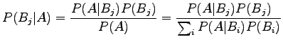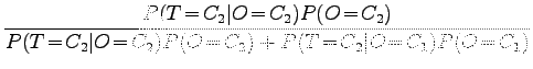
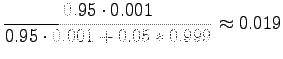
Using the theorem, the probability that the program is right, when it tells that the stem is ``siittää'', is:

$$P(O\! = C_2\vert T = C_2)$$

$$= \frac{P(T\!=\!C_2\vert O\!=\!C_2)P(O\!=\!C_2)}{P(T\!=\!C_2\vert O\!=\!C_2)P(O\!=\!C_2) + P(T\!=\!C_2\vert O\!=\!C_1)P(O\!=\!C_1)}$$

$$= \frac{0.95 \cdot 0.001}{0.95 \cdot 0.001+ 0.05 * 0.999} \approx 0.019$$

3.

To generate a one letter word, the given random language should generate two symbols, i.e. word boundary after something else. The probability for this is

$$P(s=t_1)=\frac{1}{30}\cdot \frac{1}{30}$$

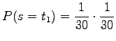and there are 29 words of this kind.

Respectively, the probability of a word of two letters is

$$P(s=t_1,t_1)=\frac{1}{30} \cdot \frac{1}{30} \cdot \frac{1}{30}$$

There are $29^2$ words of this kind. For three letter words,

$$P(s=3)=\frac{1}{30} \cdot \frac{1}{30} \cdot \frac{1}{30} \cdot \frac{1}{30}$$

and the number of words is $29^3$.

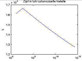
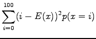
As the probability of the word is directly proportional to its expected incidence in the test data, we can make a table similar to the table 1.3 in the book by directly calculating probabilities. As words of same length have equal probability, and they cannot be sorted by frequency, we count the $k$ value for only one word per length. The results are presented in table 1 and drawn to Figure 1.

Table: Zipf constant. Left column tells the ranking number in a list sorted by frequency, middle column how many times we would expect the word to occur in a text of 1000000 words, and the right column is the product of those two.

$r$	$f$	$k$
15	1111	16111
450	37.04	16648
13064	1.235	16129
378900	0.0412	15593
1098800	0.00137	15073
318660000	0.0000457	14570

Figure: $k$ in function of $r$

We can see that the even for a random language, $k$ remains quite constant for a large range of $r$. Zipf's discovery may not seem so extraordinary in this light.

4.

In the solution it is assumed that the following formulas are known:

$$E(x) = \int_{-\infty}^\infty xp(x)dx$$

$$Var(x) = \int_{-\infty}^\infty (x-E(x))^2 p(x) dx$$

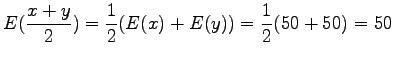
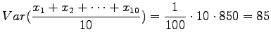
a)

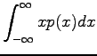
Let's calculate the expected value for one toss of the dice. Each side of the dice is of equal probability, so the probability of each event is $p(x)=\frac{1}{101}$.

Expectation value:

$$E(x) = \sum_{i=0}^{100} ip(x=i)$$

$$= \frac{1}{101}(1+2+3+4+\dots+100)$$

$$= \frac{1}{101}\left((1+100)+(2+99)+(3+98)+\dots+(50+51)\right)$$

$$= \frac{50*101}{101}=50$$

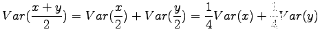
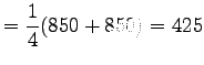
Variance:

$$Var(x) = \sum_{i=0}^{100} (i-E(x))^2p(x=i)$$

$$= \frac{1}{101}(50^2+49^2+\dots+1+0+1+2^2+\dots+49^2+50^2)$$

$$= \frac{2}{101}(1+2^2+\dots+49^2+50^2)$$

Now we can use formula

$$1+2^2+3^2+4^2+\dots+n^2=\frac{n(n+1)(2n+1)}{6}$$

to get the result:

$$Var(x) = \frac{2}{101}\frac{50\cdot 51\cdot 101}{6}=850$$

b)

To solve the problem, we will need a couple of basic formulas for probability calculation, which are derived here. (However, the derivations are not essential for the course.)

Expectation value of the sum of independent random variables

$$E(x+y) = \int (x+y)p(x,y)dxdy$$

$$= \int (x+y)p(x)p(y)dxdy$$

$$= \int xp(x)p(y)dxdy + \int yp(x)p(y)dxdy$$

$$= \int p(y)dy \int xp(x) dx +\int p(x)dx \int yp(y) dy$$

$$= 1\cdot \int xp(x) dx +1\cdot \int yp(y) dy$$

$$= E(x)+E(y)$$

Variance of a random variable multiplied by a constant

$$Var(ax) = \int (ax-E(ax))^2p(x)dx$$

$$= \int(ax-aE(x))^2p(x)dx$$

$$= a^2\int(x-E(x))^2p(x)$$

$$= a^2Var(x)$$

Variance of the sum of independent random variables

$$Var(x+y) = \int\int(x+y-E(x+y))^2p(x,y)dxdy$$

$$= \int\int(x+y)^2p(x,y)dxdy-2\int\int(x+y)E(x+y)p(x,y)dxdy$$

$$+\int\int E(x+y)^2p(x,y)dxdy$$

$$= E((x+y)^2)-2E(x+y)^2+E(x+y)^2$$

$$= E((x+y)^2)-E(x+y)^2$$

$$= E(x^2+2xy+y^2)-(E(x)+E(y))^2$$

$$= E(x^2)+E(2xy)+E(y^2)-E(x)^2-2E(x)E(y)-E(y)^2$$

$$= E(x^2)-E(x)^2 + E(y^2)-E(y)^2$$

$$+\int\int 2xyp(x)p(y)dxdy -2\int xp(x)dx\int yp(y)dy$$

$$= E(x^2)-E(x)^2 + E(y^2)-E(y)^2$$

$$= Var(x)+Var(y)$$

Now we have all the needed formulas. We want to calculate expectation value for the sum $(x+y)/2$, where $x$ is the random variable corresponding to the first throw and $y$ to the second.

$$E(\frac{x+y}{2})=\frac{1}{2}(E(x)+E(y))=\frac 12 (50 +50 ) = 50$$

We notice that the expectation value does not change. What about variance, then?

$$Var(\frac{x+y}{2})=Var(\frac x2)+Var(\frac y2)=\frac 14 Var(x)+ \frac 14 Var(y)$$

$$= \frac 14 ( 850 +850) = 425$$

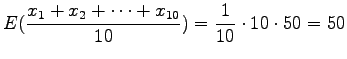
c)

We throw ten dices. Using the learned solutions:

$$E(\frac{x_1+x_2+\dots+x_{10}}{10})=\frac{1}{10}\cdot10\cdot 50= 50$$

$$Var(\frac{x_1+x_2+\dots+x_{10}}{10})= \frac {1}{100}\cdot 10 \cdot850 = 85$$

d)

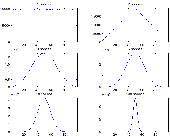
As we throw even more dices, the distribution will sharpen around the expectation value. At the inifinite, expectation value is 50 and variance 0, which means that we will always get a result of 50.

The expectation value and variance do not tell everything about the distribution. In figure 2 there are results for varying number of dice tosses simulated using Matlab. The shape of the distribution moves nearer to the normal (gaussian) distribution as the number of dices grow. This is why natural phenomena are often modelled using normal distribution: If many small random events affect to the result, it will be normal distributed. This is also is good excuse for transforming calculations to easier forms.

More formal proof for that the distribution will approach normal is found from http:// mathworld.wolfram.com/CentralLimitTheorem.html

Figure: Throwing dices. The throw was simulated million times for each curve.

5.

The goal is to minimize the total code length

$$L(x, \theta) = L(\theta) + L(x\,\vert\,\theta).$$

Let's denote the set of parameters that minimize the previous expression as $\hat{\theta}$:

$$\hat{\theta} = \argmin_{\theta} L(x, \theta) = \argmin_{\theta} \{L(\theta) + L(x\,\vert\,\theta) \}.$$

Now we substitute the code lengths for their optimal values $L(\theta) = -\log p(\theta)$ and $L(x\,\vert\,\theta) = -\log p(x\,\vert\,\theta)$:

$$\hat{\theta} = \argmin_{\theta} \{-\log p(\theta) - \log p(x\,\vert\,\theta) \}$$

The logarithmic terms can be combined using the product rule of logarithms:

$$\hat{\theta} = \argmin_{\theta} \{-\log( p(\theta) p(x\,\vert\,\theta) ) \}$$

As logarithm is a monotonically increasing function, and thus its complement monotonically decreasing, the minimum can be obtained by maximixing the product of the two probabilities:

$$\hat{\theta} = \argmax_{\theta} \{ p(\theta) p(x\,\vert\,\theta) \}$$

Finally, from Bayes' theorem we get $p(x, \theta) = p(x) p(\theta\,\vert\,x) = p(\theta) p(x\,\vert\,\theta)$:

$$\hat{\theta} = \argmax_{\theta} \{ p(x) p(\theta\,\vert\,x) \}$$

Probability $p(x)$ does not depend on the parameters, so we can leave it out. Thus we see that the same goal is obtained by maximizing the posterior distribution of the model:

$$\hat{\theta} = \argmax_{\theta} p(\theta\,\vert\,x)$$