T-61.5020 Statistical Natural Language Processing
Answers 3 -- Information retrieval
Version 1.1

1.
Let's modify the given table to a format that suits better the first calculations.

Table: Modified tables. (tp = True Positives, fp = False Positives, fn = False Negatives, fp = True Negatives)
engine 1 relevant non-relevant
returned 4 tp 6 fp
not returned 2 fn 9988 tn
engine 2 relevant non-relevant
returned 6 tp 4 fp
not returned 0 fn 9990 tn


In the following table there are the definitions of the five first measures and the results for applying them.

Table: Results. Note that only the precision and recall values are in a region that is easy to understand.
measure $ \textrm{definition}\!\!$ $ \textrm{engine 1}\!\! $ $ \textrm{engine 2}\!\! $ Ratio of
precision $ \frac{tp}{tp+fp} $ $ \frac{4}{4+6}=40\%
$ $ \frac{6}{6+4}=60\% $ relevants in returned
recall $ \frac{tp}{tp+fn} $ $ \frac{4}{4+2}=67\%
$ $ \frac{6}{6+0}=100\% $ relevants found
fallout $ \frac{fp}{fp+tn} $ $ \frac{6}{6+9988}=0.06\%
$ $ \frac{4}{4+9990}=0.04\% $ returned non-relevants
accuracy $ \frac{tp+tn}{N} $ $ \frac{4+9988}{10000}=99.92\%\!\!
$ $ \frac{6+9990}{10000}=99.96\%\!\!$ correctly classified
error $ \frac{fp+fn}{N} $ $ \frac{6+2}{10000}=0.08\%
$ $ \frac{4}{10000}=0.04\% $ incorrectly classified


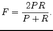
F-measure is defined using both the precision and recall:
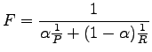
$\displaystyle F = \frac{1}{\alpha\frac1P+ (1-\alpha)\frac1R}$    

where $ P$ stands for precision and $ R$ recall. $ \alpha$ controls the weighting between them. If we choose $ \alpha=0.5$,

$\displaystyle F = \frac{2PR}{P+R}.$    

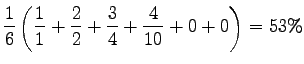
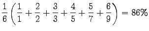
For the first engine $ F_1=50\%$ and for the second $ F_2=75\%$.

When calculating uninterpolated average precision, we go through the list of returned documents, and whenever a relevant document is seen, we calculate the precision over the documents processed so far. Relevants that were not returned are taken into account with a zero precision. Then we take an average over the precisions.


$\displaystyle \textrm{UAP}_1$ $\displaystyle =$ $\displaystyle \frac16 \left(\frac11 +\frac 22 + \frac34
+\frac4{10} + 0 + 0 \right) = 53 \%$  
$\displaystyle \textrm{UAP}_2$ $\displaystyle =$ $\displaystyle \frac16 \left(\frac11 +\frac 22 + \frac33 +\frac4{5} +\frac5{7}
+\frac{6}{9}\right) = 86 \%$  

2.
Word frequences in the documents were given: $ df_1=21$ and $ df_2=500$. The total number of the documents is $ N=10000$. Inverser Document Frequency is defined as $ IDF_i=\log_2 \frac{N}{df_i}$, so for the word $ w_1$ it is $ \log_2 \frac{10000}{21}=8.9$ and for the word $ w_2$ $ \log_2 \frac{10000}{500}=4.3$. Thus the first word got almost twice the weight of the second word.

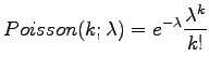
The idea in Residual Inverse Document Frequency (RIDF) is that we can model the occurrences of a word using a Poisson distribution. This works well for words that are evenly distributed in a corpus. Contentually important words usually occur in groups inside the documents that discuss the corresponding matter, and therefore Poisson distribution gives an incorrect estimation for their frequencies. In RIDF we measure the difference between IDF and Poisson distributions. The more difference we have, the more does the word tell about the document. (Note: There are many errors in this section of the course book's first edition.)

Actual calculations are the following: On average, word $ w_i$ occurs $ \lambda=\frac{cf_i}{N}$ times in a document. The probability for that in a certain document word $ w_1$ occur $ k$ times is obtained from the Poisson distribution:
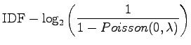
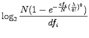
$\displaystyle Poisson(k;\lambda)=e^{-\lambda} \frac{\lambda^k}{k!}$    

RIDF is defined as

$\displaystyle \textrm{RIDF}=\textrm{IDF} - \log_2\left( \frac 1{1-Poisson(0,\lambda)} \right).$      

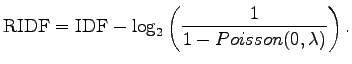
I.e., we take from the Poisson distribution the probability that the word occurs at least once in the document ( $ 1-Poisson(0,\lambda$)). IDF, on the other hand, was based on the observed value of that probability ( $ \frac{df_i}{N}$).

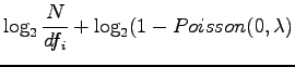
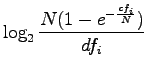
Simplifying the expression of RIDF:

$\displaystyle \textrm{RIDF}$ $\displaystyle =$ $\displaystyle \textrm{IDF} - \log_2\left( \frac
1{1-Poisson(0,\lambda)} \right)$  
  $\displaystyle =$ $\displaystyle \log_2 \frac{N}{df_i}+\log_2 (1-Poisson(0,\lambda)$  
  $\displaystyle =$ $\displaystyle \log_2 \frac{N(1-e^{-\frac{cf_i}N(\frac{\lambda}{0!})^0})}{df_i}$  
  $\displaystyle =$ $\displaystyle \log_2 \frac{N(1-e^{-\frac{cf_i}N})}{df_i}$  

Assigning the values:
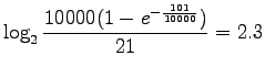
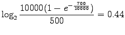
$\displaystyle \textrm{RIDF}_1$ $\displaystyle =$ $\displaystyle \log_2 \frac{10000(1-e^{-\frac{101}{10000}})}{21} = 2.3$  
$\displaystyle \textrm{RIDF}_2$ $\displaystyle =$ $\displaystyle \log_2 \frac{10000(1-e^{-\frac{700}{10000}})}{500} = 0.44$  

We see that RIDF weighted the word $ w_1$ 2.5 times more than IDF. Thus both methods estimate that $ w_1$ is a more relevant search term than $ w_2$.

3.
The asked document-word matrix is presented in table 3.

Table: Document-word matrix
  $ d_1$ $ d_2$ $ d_3$ $ d_4$ $ d_5$ $ d_6$ $ d_7$
Schumacher 0 1 0 1 0 0 0
rata 1 1 1 0 0 1 0
formula 1 0 1 1 0 0 0
kolari 0 0 1 1 0 0 0
galaksi 0 0 0 0 1 1 0
tähti 0 0 1 0 0 1 1
planeetta 0 0 0 0 0 1 1
meteoriitti 0 0 0 0 1 0 0


In Singular Value Decomposition (SVD) we decompose the matrix $ A$ as:

$\displaystyle A=USV^T$    

Here $ U$ is an orthogonal $ m \times n$ matrix, $ S$ is a diagonal $ n \times n$ matrix and $ V$ an orthogonal $ n \times n$ matrix. The matrices are presented in tables 4, 5, and 6.


Table: $ U$
  $ dim_1$ $ dim_2$ $ dim_3$ $ dim_4$ $ dim_5$ $ dim_6$ $ dim_7$ $ dim_8$
Schumacher -0.200 -0.336 0.290 0.115 0.823 0.007 0.121 -0.243
rata -0.590 0.007 0.184 0.686 -0.232 -0.183 0.025 0.243
formula -0.435 -0.464 -0.040 -0.225 -0.333 0.609 0.045 -0.243
kolari -0.317 -0.361 -0.108 -0.494 0.071 -0.438 -0.285 0.485
galaksi -0.200 0.400 0.602 -0.242 -0.053 0.028 -0.563 -0.243
tähti -0.464 0.376 -0.408 -0.213 0.034 -0.345 0.275 -0.485
planeetta -0.257 0.476 -0.234 -0.070 0.363 0.530 -0.007 0.485
meteoriitti -0.026 0.116 0.534 -0.336 -0.132 -0.048 0.713 0.243


Table: $ S$
2.949 0 0 0 0 0 0
0 2.107 0 0 0 0 0
0 0 1.459 0 0 0 0
0 0 0 1.311 0 0 0
0 0 0 0 1.183 0 0
0 0 0 0 0 0.638 0
0 0 0 0 0 0 0.460
0 0 0 0 0 0 0


Table: $ V$
  $ d_1$ $ d_2$ $ d_3$ $ d_4$ $ d_5$ $ d_6$ $ d_7$
$ dim_1$ -0.348 -0.217 0.099 0.352 -0.478 0.669 0.152
$ dim_2$ -0.268 -0.156 0.325 0.611 0.499 -0.275 0.316
$ dim_3$ -0.613 -0.210 -0.255 -0.187 -0.390 -0.559 0.130
$ dim_4$ -0.323 -0.551 0.098 -0.460 0.474 0.279 -0.261
$ dim_5$ -0.077 0.245 0.779 -0.440 -0.157 -0.030 0.328
$ dim_6$ -0.512 0.598 0.099 0.124 0.094 0.048 -0.587
$ dim_7$ -0.244 0.404 -0.440 -0.216 0.335 0.290 0.583


Table: Scaled $ B$
  $ d_1$ $ d_2$ $ d_3$ $ d_4$ $ d_5$ $ d_6$ $ d_7$
$ dim_1$ -0.913 -0.924 -0.971 -0.634 -0.400 -0.768 -0.646
$ dim_2$ -0.407 -0.384 -0.238 -0.773 0.917 0.640 0.764


Table: Correlations of documents
  $ d_1$ $ d_2$ $ d_3$ $ d_4$ $ d_5$ $ d_6$ $ d_7$
$ d_1$ 1.000            
$ d_2$ 1.000 1.000          
$ d_3$ 0.984 0.988 1.000        
$ d_4$ 0.894 0.882 0.800 1.000      
$ d_5$ -0.008 0.018 0.171 -0.455 1.000    
$ d_6$ 0.441 0.464 0.594 -0.008 0.894 1.000  
$ d_7$ 0.279 0.304 0.446 -0.180 0.958 0.985 1.000


We reduce the inner dimension to two by taking only the two largest eigenvalues from $ S$ and leaving the rest of the dimensions out from the matrices $ U$ and $ V$. Now the similarity of the documents can be compared using the matrix $ B=SV^T$. If $ B$'s columns are scaled to unity, it is easy to calculate correlations between rows. This kind of a scaled matrix is in table 7. (Similarity of words could be compared from $ W=US$.) From the correlation matrix (table 8) we see that the Formula 1 and astronomy related articles correlate much more inwardly than crosswise. Documents $ d_5$ and $ d_7$ that were totally uncorrelated before, are now clearly correlated. We have projected the data to two-dimensional space, and similar articles have ended up near each other in that reduced dimension.


svirpioj[a]cis.hut.fi